Income and Expenditures in the US

Description

Personal income and personal consumption expenditures in the US between January 1959 and February 2001 (seasonally adjusted at annual rates).

Usage

data("USIncExp")

Format

A multivariate monthly time series from 1959(1) to 2001(2) with variables

income

monthly personal income (in billion US dollars),

expenditure

monthly personal consumption expenditures (in billion US Dollars).

Source

Economagic

References

A. Zeileis, F. Leisch, K. Hornik, C. Kleiber (2002), strucchange: An R Package for Testing for Structural Change in Linear Regression Models. Journal of Statistical Software 7(2), 1–38.

Examples

library("strucchange")

## These example are presented in the vignette distributed with this
## package, the code was generated by Stangle("strucchange-intro.Rnw")

###################################################
### chunk number 1: data
###################################################
library("strucchange")
data("USIncExp")
plot(USIncExp, plot.type = "single", col = 1:2, ylab = "billion US$")
legend(1960, max(USIncExp), c("income", "expenditures"),
       lty = c(1,1), col = 1:2, bty = "n")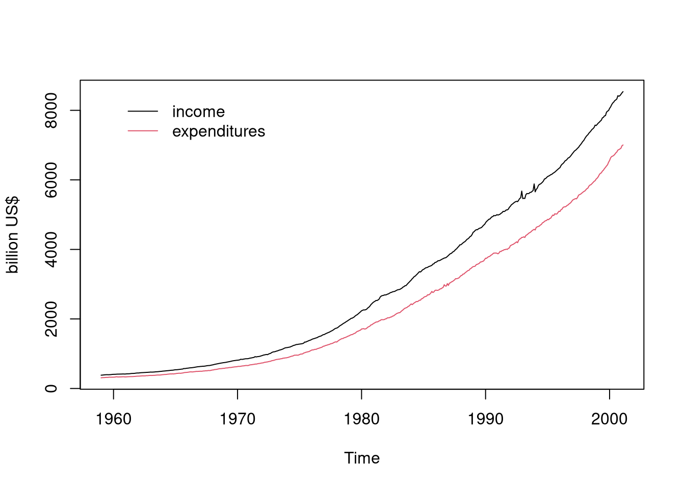

###################################################
### chunk number 2: subset
###################################################
library("strucchange")
data("USIncExp")
USIncExp2 <- window(USIncExp, start = c(1985,12))


###################################################
### chunk number 3: ecm-setup
###################################################
coint.res <- residuals(lm(expenditure ~ income, data = USIncExp2))
coint.res <- lag(ts(coint.res, start = c(1985,12), freq = 12), k = -1)
USIncExp2 <- cbind(USIncExp2, diff(USIncExp2), coint.res)
USIncExp2 <- window(USIncExp2, start = c(1986,1), end = c(2001,2))
colnames(USIncExp2) <- c("income", "expenditure", "diff.income",
                         "diff.expenditure", "coint.res")
ecm.model <- diff.expenditure ~ coint.res + diff.income


###################################################
### chunk number 4: ts-used
###################################################
plot(USIncExp2[,3:5], main = "")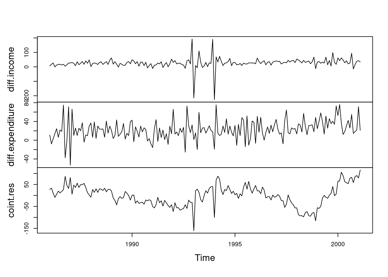

###################################################
### chunk number 5: efp
###################################################
ocus <- efp(ecm.model, type="OLS-CUSUM", data=USIncExp2)
me <- efp(ecm.model, type="ME", data=USIncExp2, h=0.2)


###################################################
### chunk number 6: efp-boundary
###################################################
bound.ocus <- boundary(ocus, alpha=0.05)


###################################################
### chunk number 7: OLS-CUSUM
###################################################
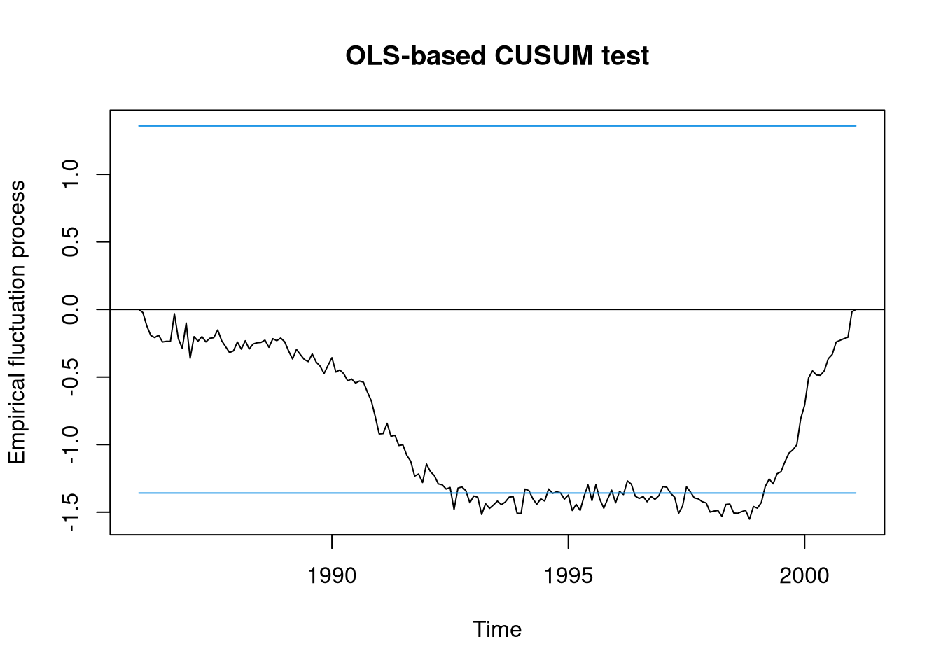
plot(ocus)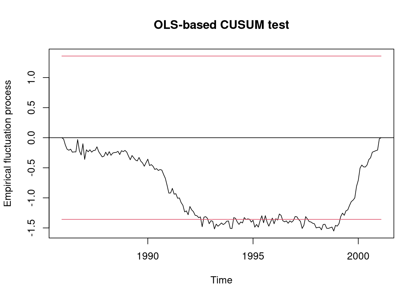

###################################################
### chunk number 8: efp-boundary2
###################################################
plot(ocus, boundary = FALSE)
lines(bound.ocus, col = 4)
lines(-bound.ocus, col = 4)

###################################################
### chunk number 9: ME-null
###################################################
plot(me, functional = NULL)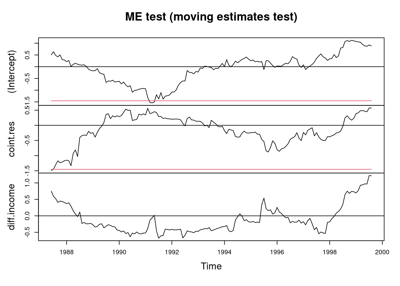

###################################################
### chunk number 10: efp-sctest
###################################################
sctest(ocus)

    OLS-based CUSUM test

data:  ocus
S0 = 1.5511, p-value = 0.01626

###################################################
### chunk number 11: efp-sctest2
###################################################
sctest(ecm.model, type="OLS-CUSUM", data=USIncExp2)

    OLS-based CUSUM test

data:  ecm.model
S0 = 1.5511, p-value = 0.01626

###################################################
### chunk number 12: Fstats
###################################################
fs <- Fstats(ecm.model, from = c(1990, 1), to = c(1999,6), data = USIncExp2)


###################################################
### chunk number 13: Fstats-plot
###################################################
plot(fs)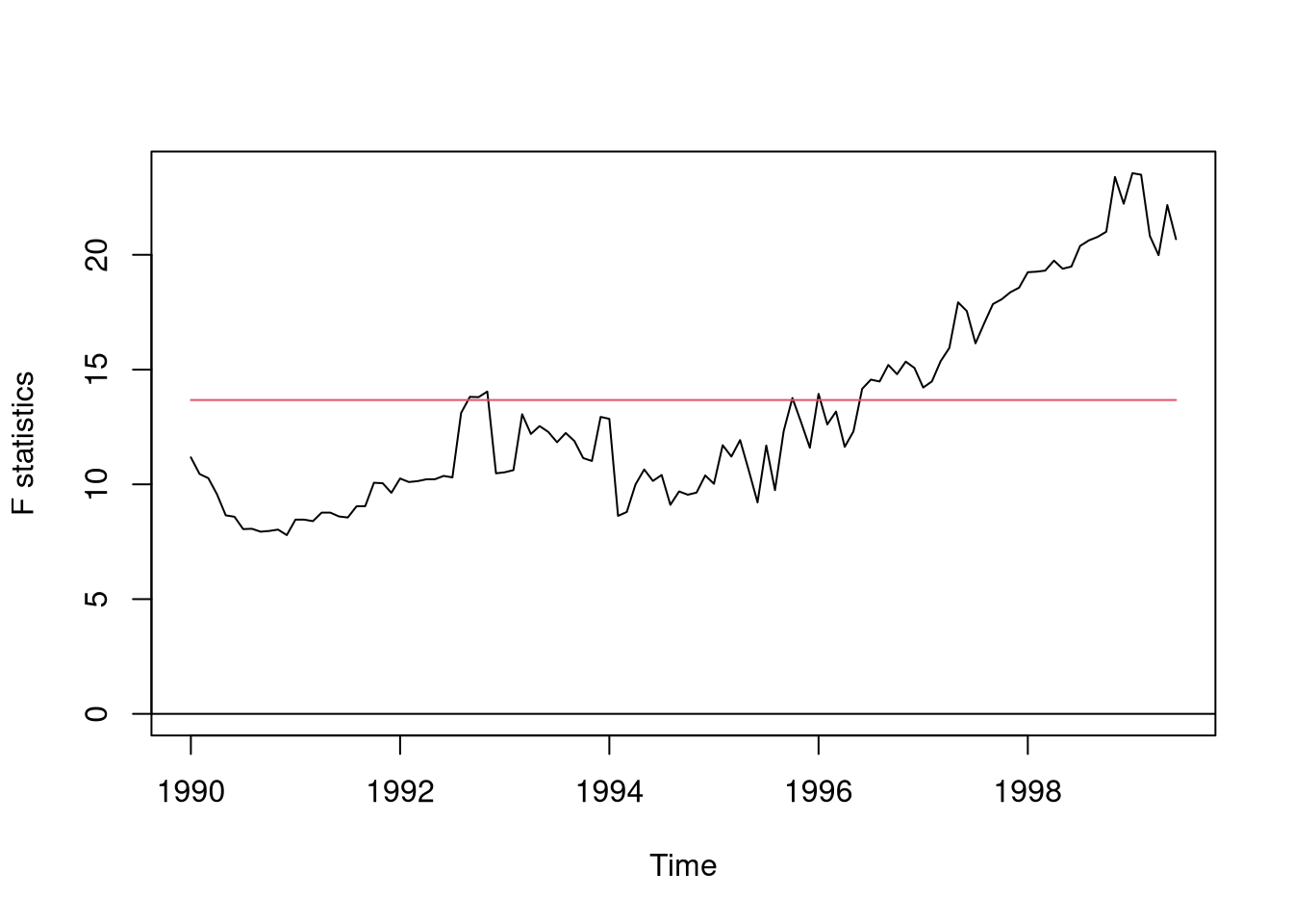

###################################################
### chunk number 14: pval-plot
###################################################
plot(fs, pval=TRUE)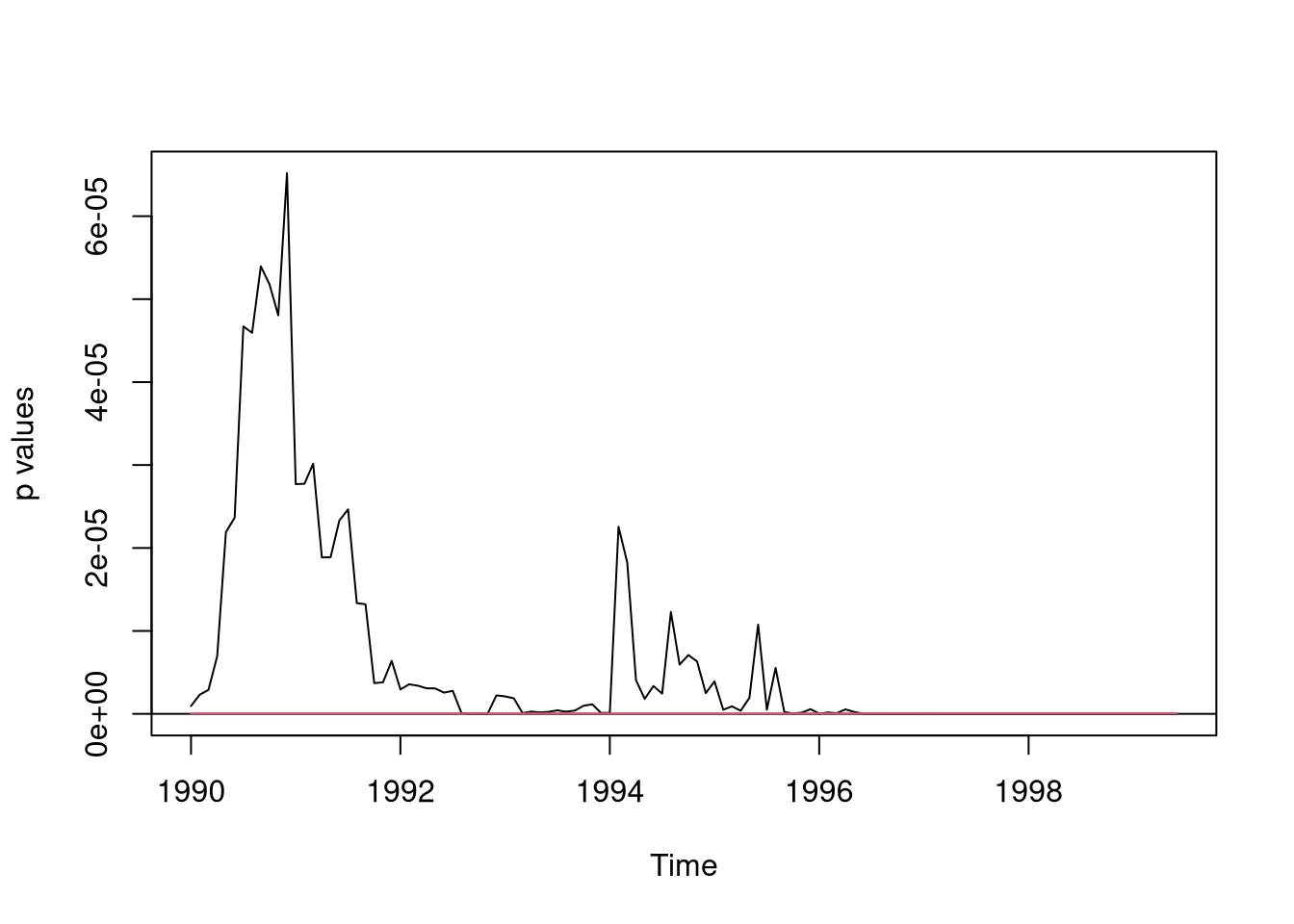

###################################################
### chunk number 15: aveF-plot
###################################################
plot(fs, aveF=TRUE)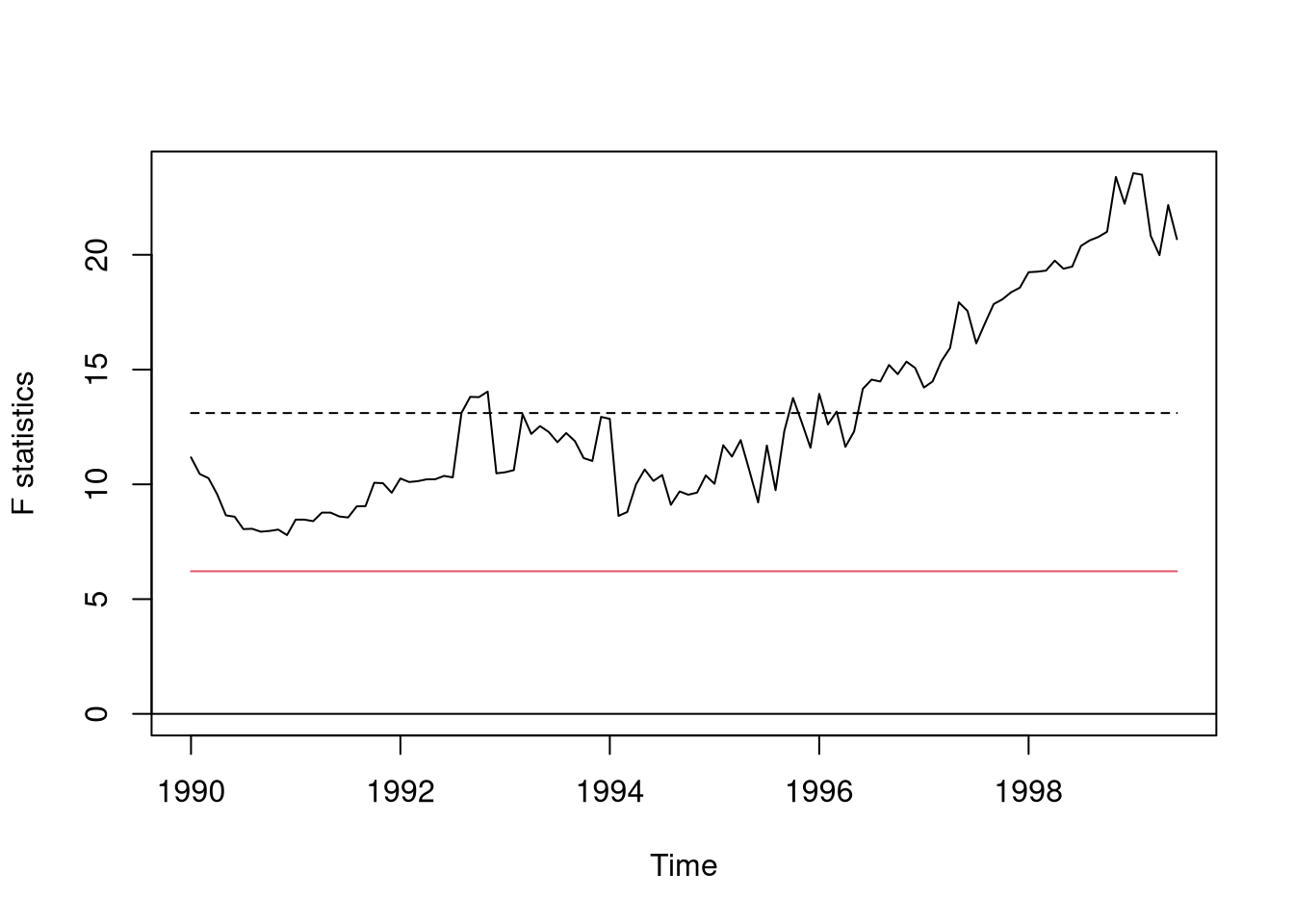

###################################################
### chunk number 16: Fstats-sctest
###################################################
sctest(fs, type="expF")

    expF test

data:  fs
exp.F = 8.9955, p-value = 0.001311

###################################################
### chunk number 17: Fstats-sctest2
###################################################
sctest(ecm.model, type = "expF", from = 49, to = 162, data = USIncExp2)

    expF test

data:  ecm.model
exp.F = 8.9955, p-value = 0.001311

###################################################
### chunk number 18: mefp
###################################################
USIncExp3 <- window(USIncExp2, start = c(1986, 1), end = c(1989,12))
me.mefp <- mefp(ecm.model, type = "ME", data = USIncExp3, alpha = 0.05)


###################################################
### chunk number 19: monitor1
###################################################
USIncExp3 <- window(USIncExp2, start = c(1986, 1), end = c(1990,12))
me.mefp <- monitor(me.mefp)


###################################################
### chunk number 20: monitor2
###################################################
USIncExp3 <- window(USIncExp2, start = c(1986, 1))
me.mefp <- monitor(me.mefp)

Break detected at observation # 72 

me.mefp

Monitoring with ME test (moving estimates test) 

Initial call:
  mefp.formula(formula = ecm.model, type = "ME", data = USIncExp3,      alpha = 0.05) 

Last call:
  monitor(obj = me.mefp) 

Significance level   :  0.05 
Critical value       :  3.109524 
History size         :  48 
Last point evaluated :  182 
Structural break at  :  72 

Parameter estimate on history :
(Intercept)   coint.res diff.income 
 18.9299679  -0.3893141   0.3156597 
Last parameter estimate :
(Intercept)   coint.res diff.income 
27.94869106  0.00983451  0.13314662 

###################################################
### chunk number 21: monitor-plot
###################################################
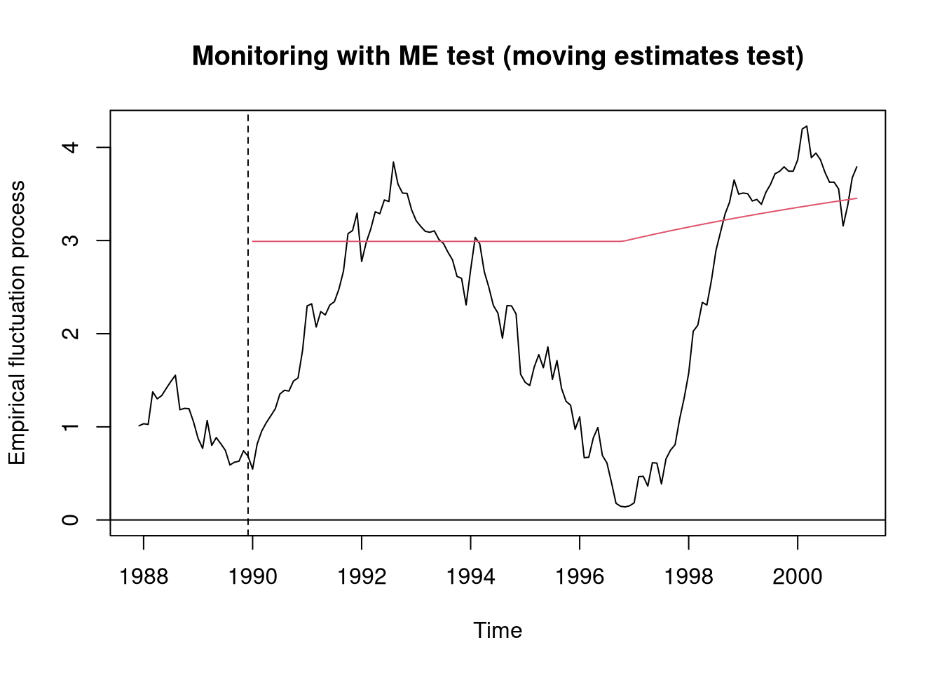
plot(me.mefp)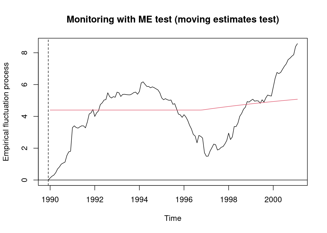

###################################################
### chunk number 22: mefp2
###################################################
USIncExp3 <- window(USIncExp2, start = c(1986, 1), end = c(1989,12))
me.efp <- efp(ecm.model, type = "ME", data = USIncExp3, h = 0.5)
me.mefp <- mefp(me.efp, alpha=0.05)


###################################################
### chunk number 23: monitor3
###################################################
USIncExp3 <- window(USIncExp2, start = c(1986, 1))
me.mefp <- monitor(me.mefp)

Break detected at observation # 70 

###################################################
### chunk number 24: monitor-plot2
###################################################
plot(me.mefp)