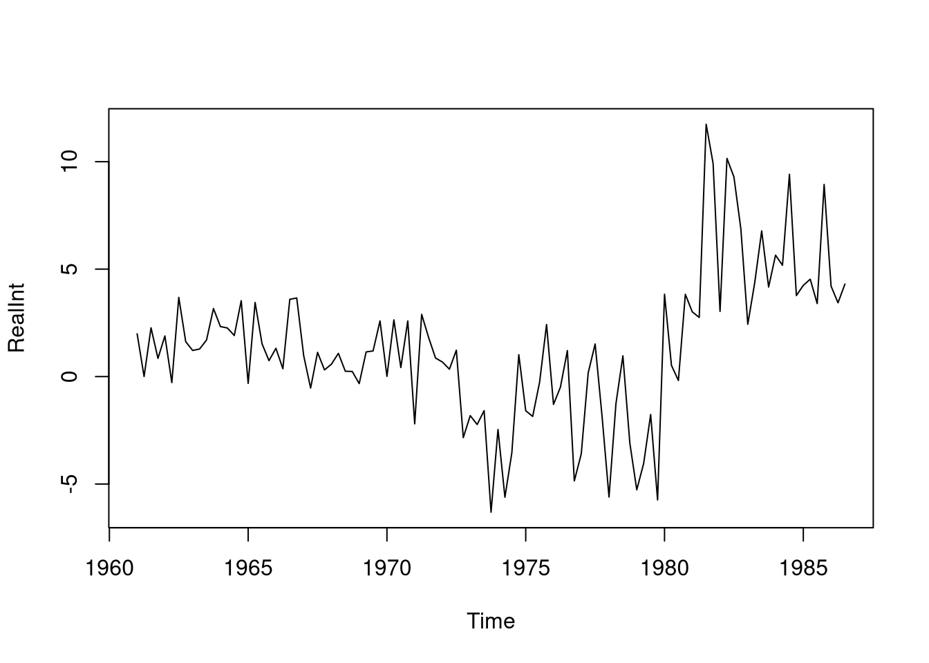
US Ex-post Real Interest Rate
Description
US ex-post real interest rate: the three-month treasury bill deflated by the CPI inflation rate.
References
Bai J., Perron P. (2003), Computation and Analysis of Multiple Structural Change Models, Journal of Applied Econometrics, 18, 1-22.
Zeileis A., Kleiber C. (2005), Validating Multiple Structural Change Models - A Case Study. Journal of Applied Econometrics, 20, 685-690.
Examples
## estimate breakpoints
bp.ri <- breakpoints(RealInt ~ 1, h = 15)
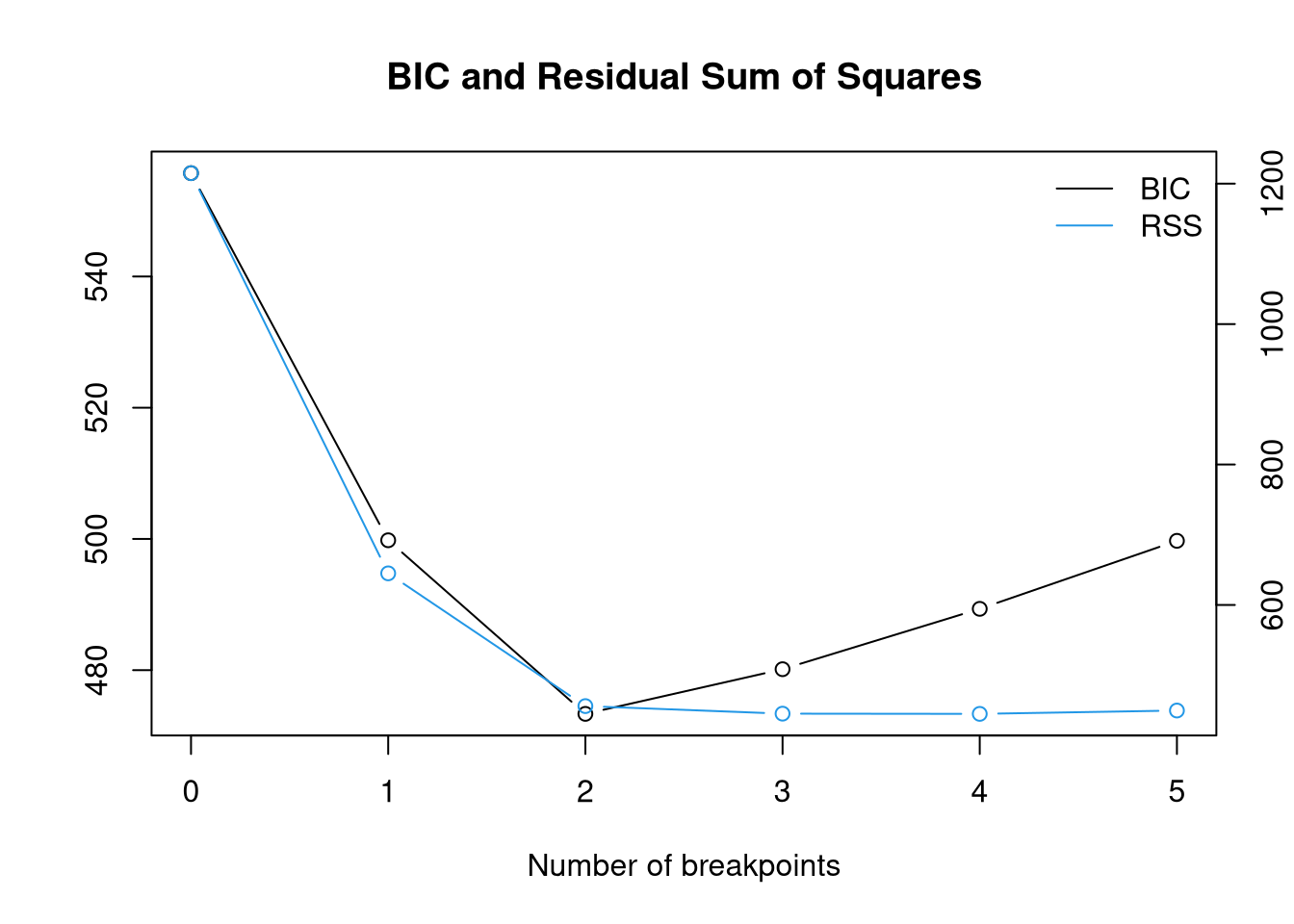
plot(bp.ri)
     Optimal (m+1)-segment partition:

Call:
breakpoints.formula(formula = RealInt ~ 1, h = 15)

Breakpoints at observation number:

m = 1               79
m = 2         47    79
m = 3      24 47    79
m = 4      24 47 64 79
m = 5   16 31 47 64 79

Corresponding to breakdates:

m = 1                                   1980(3)
m = 2                   1972(3)         1980(3)
m = 3           1966(4) 1972(3)         1980(3)
m = 4           1966(4) 1972(3) 1976(4) 1980(3)
m = 5   1964(4) 1968(3) 1972(3) 1976(4) 1980(3)

Fit:

m   0      1      2      3      4      5
RSS 1214.9  645.0  456.0  445.2  444.9  449.6
BIC  555.7  499.8  473.3  480.1  489.3  499.7
## fit segmented model with three breaks
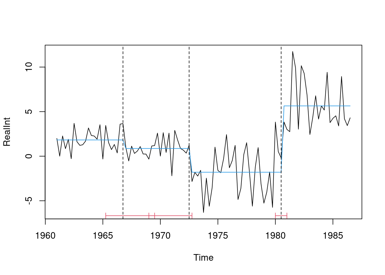
fac.ri <- breakfactor(bp.ri, breaks = 3, label = "seg")
fm.ri <- lm(RealInt ~ 0 + fac.ri)
summary(fm.ri)
Call:
lm(formula = RealInt ~ 0 + fac.ri)

Residuals:
    Min      1Q  Median      3Q     Max
-4.5157 -1.3674 -0.0578  1.3248  6.0990

Coefficients:
           Estimate Std. Error t value Pr(>|t|)
fac.riseg1   1.8236     0.4329   4.213 5.57e-05 ***
fac.riseg2   0.8661     0.4422   1.959    0.053 .
fac.riseg3  -1.7961     0.3749  -4.791 5.83e-06 ***
fac.riseg4   5.6429     0.4329  13.036  < 2e-16 ***
---
Signif. codes:  0 '***' 0.001 '**' 0.01 '*' 0.05 '.' 0.1 ' ' 1

Residual standard error: 2.121 on 99 degrees of freedom
Multiple R-squared:  0.6842,    Adjusted R-squared:  0.6714
F-statistic: 53.62 on 4 and 99 DF,  p-value: < 2.2e-16
## setup kernel HAC estimator
vcov.ri <- function(x, ...) kernHAC(x, kernel = "Quadratic Spectral",
  prewhite = 1, approx = "AR(1)", ...)

## Results from Table 1 in Bai & Perron (2003):
## coefficient estimates
coef(bp.ri, breaks = 3)
                  (Intercept)
1961(1) - 1966(4)   1.8236167
1967(1) - 1972(3)   0.8660848
1972(4) - 1980(3)  -1.7961384
1980(4) - 1986(3)   5.6428896
## corresponding standard errors
sapply(vcov(bp.ri, breaks = 3, vcov = vcov.ri), sqrt)
1961(1) - 1966(4) 1967(1) - 1972(3) 1972(4) - 1980(3) 1980(4) - 1986(3)
        0.1857577         0.1499849         0.5026749         0.5887460
## breakpoints and confidence intervals
confint(bp.ri, breaks = 3, vcov = vcov.ri)
     Confidence intervals for breakpoints
     of optimal 4-segment partition:

Call:
confint.breakpointsfull(object = bp.ri, breaks = 3, vcov. = vcov.ri)

Breakpoints at observation number:
  2.5 % breakpoints 97.5 %
1    18          24     35
2    33          47     48
3    77          79     81

Corresponding to breakdates:
  2.5 %   breakpoints 97.5 %
1 1965(2) 1966(4)     1969(3)
2 1969(1) 1972(3)     1972(4)
3 1980(1) 1980(3)     1981(1)