Testing, Monitoring, and Dating Structural Changes in the UK Seatbelt Data
A Hands-On Overview of the R Package strucchange
Abstract
An overview of the R package strucchange is provided using a hands-on tutorial based on the classic UK seatbelt data. The underlying inference methods are only briefly motivated with minimal mathematical notation. More theoretical details can be found in the references.
Introduction
The R package strucchange was first introduced as a comprehensive toolbox for testing, monitoring, and dating structural changes in linear regression models. Later on, many of the methods have been generalized to any parametric model estimated by least squares, maximum likelihood, and other M-type estimators. In short, these methods are concerned with answering the following questions.
- Testing: Are the parameters of a model stable throughout the sample period or is there evidence that they changed over time?
- Monitoring: If a model with stable parameters could be established, do the parameters remain stable as new observations come in?
- Dating: If there is evidence for changes in the parameters, when and how did the parameters change?
Zeileis et al. (2002) introduced the testing and monitoring functionality for linear regression models which was supplemented by the corresponding dating techniques in Zeileis et al. (2003).
Zeileis (2005) and Zeileis and Hornik (2007) showed that tests based on the model scores offer a unified framework that can also be applied to general parametric models with M-type estimators (least squares, maximum likelihood, instrumental variables, robust M-estimation, …). Based on these ideas Zeileis (2006) introduces an object-oriented implementation that facilitates parameter stability tests far beyond the original scope of linear time series models. For example, the tests are also used for cross-section data to assess parameter stability along continuous, ordinal, or categorical variables such as age, educational degree, or gender. Prominent use cases are model-based recursive partitioning (also known as regression trees) as introduced by Zeileis et al. (2008), or measurement invariance tests in psychometric models (see Merkle and Zeileis 2013).
In the following, we illustrate all of these methods from the strucchange package with a well-known data set, the so-called UK Seatbelt Data. This is a monthly time series of car drivers in Great Britain killed or seriously injured from January 1969 to December 1984. Compulsory wearing of seatbelts was introduced in the UK on January 31, 1983, and Harvey and Durbin (1986) famously analyzed the effects of this intervention using structural time series models and structural change tests.
In our analysis below, a simple seasonal autoregressive model with one lag and one seasonal lag is employed, fitted by ordinary least squares (OLS). This reveals (at least) two breakpoints: one in 1973 associated with the oil crisis and one in 1983 due to the introduction of compulsory wearing of seatbelts. However, except for the monitoring illustration no prior knowledge about either of these breaks is assumed but the breaks are identified in a data-driven way.
Data
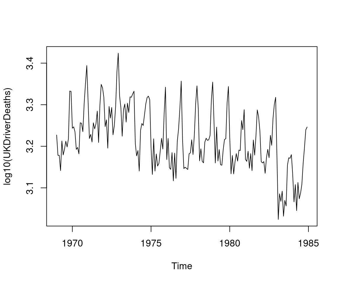
The data is available in base R under the name UKDriverDeaths and can be visualized in (decadic) logarithms as follows:
Eyeballing the time series plot already suggests that there are at least two structural changes, but it also conveys that there is considerable autocorrelation and seasonality. Thus, a model is required that can capture the autocorrelation and seasonality and then the stability of the parameters of this model can be assessed.
Base model
In our analysis below, we employ a SARIMA\((1,0,0)(1,0,0)_{12}\) model, i.e., an autoregressive model with one lag and one seasonal lag in order to capture the autocorrelation and seasonality. Doing so via least squares estimation facilitates the application of all the linear regression tests available in strucchange.
To facilitate estimating the model using lm() in base R as well as using the strucchange functions, the data is preprocessed as follows. The UKDriverDeaths time series (base ts object) is converted to a zoo series (Zeileis and Grothendieck 2005) in order to leverage some convenience functions from zoo: We take decadic logarithms, compute all required lags (0 for the response and 1 and 12 for the regressors), set short descripitive names, trim the leading and trailing missing values created by the lags (NAs), and then convert back to ts.
The SARIMA model can then be fitted to the full sample using lm().
m <- lm(y ~ ylag1 + ylag12, data = seatbelt)
summary(m)
##
## Call:
## lm(formula = y ~ ylag1 + ylag12, data = seatbelt)
##
## Residuals:
##      Min       1Q   Median       3Q      Max
## -0.14218 -0.03413  0.00614  0.03163  0.08186
##
## Coefficients:
##             Estimate Std. Error t value Pr(>|t|)
## (Intercept)   0.1826     0.1578    1.16     0.25
## ylag1         0.4310     0.0533    8.09  9.1e-14 ***
## ylag12        0.5112     0.0565    9.04  2.7e-16 ***
## ---
## Signif. codes:  0 '***' 0.001 '**' 0.01 '*' 0.05 '.' 0.1 ' ' 1
##
## Residual standard error: 0.0432 on 177 degrees of freedom
## Multiple R-squared:  0.677,  Adjusted R-squared:  0.673
## F-statistic:  185 on 2 and 177 DF,  p-value: <2e-16
To introduce a little bit of notation for this, the model above is a special case of the standard linear regression model
\[ y_i ~=~ x_i^\top \beta \; + \; \varepsilon_i \]
where \(i = 1, \dots, n\) denotes the time index, the regressor vector \(x_i\) comprises an intercept along with the two lagged series, \(\beta\) is the corresponding vector of coefficients, and \(\varepsilon_i\) has error variance \(\sigma^2\). As in most linear regression setups, the error variance is treated as a nuisance parameter and only the stability of \(\beta\) is assessed in the following sections.
Testing: Empirical fluctuation processes
As outlined in the introduction, the question that testing for structural changes is concerned with is the following.
Given that a model with parameter \(\widehat \beta\) has been estimated for all \(n\) observations, the question is whether this is appropriate or:
Are the parameters stable or did they change through the sample period \(i = 1, \dots, n\)?
In more formal notation this means that the following null hypothesis should be tested
\[ H_0:~ \beta_i = \beta_0 \qquad (i = 1, \dots, n) \]
against the alternative that \(\beta_i\) varies over time \(i\). Various patterns of deviation from \(H_0\) are conceivable, e.g., single or multiple breaks (i.e., abrupt shifts), random walks, etc.
The first family of tests discussed in this section or tests based on so-called empirical fluctuation processes. The idea of these tests is to assess the fluctuation in measures of model deviation over time by using partial sums of:
- Residuals (e.g., OLS, recursive).
- Scores (i.e., contributions to the gradient of the objective function).
- Parameter estimates (e.g., in a recursively growing or rolling time window).
For both cumultative or moving sums of these quantities, the theoretical limiting process of the empirical fluctuation process is known under the null hypothesis. It is typically some functional of a Brownian motion or Brownian bridge.
Boundaries can be chosen which are crossed by the limiting process (or some transformation of it) only with a known probability \(\alpha\), typically 5% by default.
Thus, if the empirical fluctuation process crosses the theoretical boundaries the fluctuation is improbably large and the null hypothesis of parameter stability has to be rejected.
In strucchange, the function efp() computes various CUSUM (cumulative sum) or MOSUM (moving sum) processes based on recursive or OLS residuals, parameter estimates, or scores. Significance tests can then be performed graphically by the plot() method while statistic and \(p\)-value are computed by the sctest() method. For example, the recursive estimates (RE) test for the seatbelt data yields the following output.
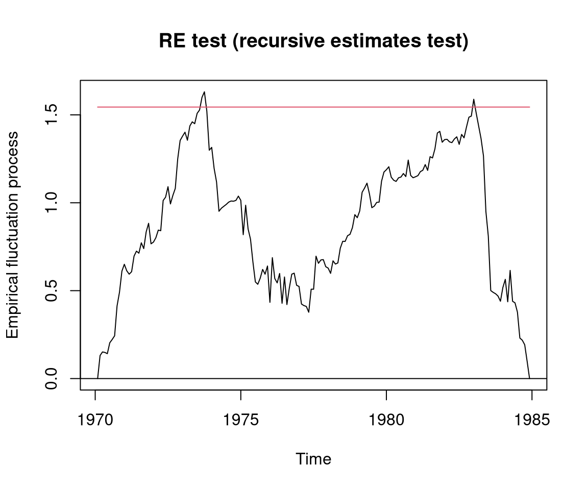
The \(p\)-value is significant at 5% level, thus providing evidence for structural changes in the parameters of the SARIMA model. What is more interesting, though, is the pattern in the RE fluctuation process that clearly shows two peaks. This conveys that there might have been two abrupt shifts in the parameters in about 1973 and 1983.
Testing: \(F\) statistics
An alternative family of parameter stability tests, that is similar in spirit to the fluctuation tests, are tests based on \(F\) statistics for a (single) break alternative. Again, a sequence is computed over all time points with an \(F\) statistic assessing the difference of the parameter estimates before and after the time point. The corresponding test procedure would then reject again if the maximum (or another functional of the \(F\) statistic sequence) exceeds a certain boundary or critical value.
In strucchange the functions Fstats() computes the sequence of \(F\) statistics with a certain trimming at the beginning and end. The significance tests can again be performed graphically by the plot() method or test statistic and \(p\)-value can be computed by the sctest() method.
The R code below uses a 10% trimming for the seatbelt data, corresponding to a sequence of \(F\) statistics from 1971(6) to 1983(6).
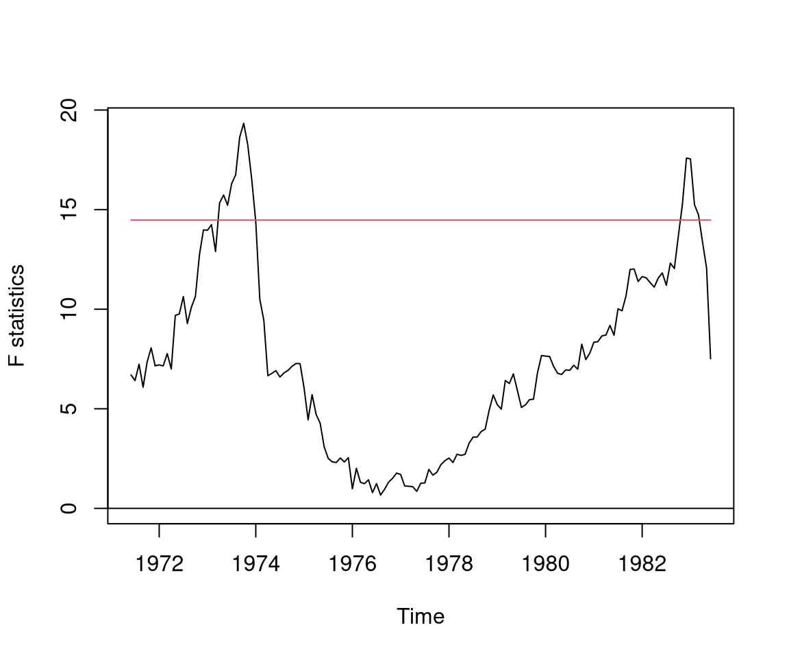
By default the maximum (or supremum) of the \(F\) statistics is used as the test statistic (sup\(F\)), yielding an even lower \(p\)-value for the seatbelt data. Again, the pattern of the \(F\) statistic sequence suggests two rather abrupt breaks in about 1973 and 1983, respectively.
Testing: Generalized empirical fluctuation processes
While the tests implemented in efp() and Fstats() in strucchange are specific to linear regression models, there is also an object-oriented implementation of so-called generalized empirical fluctuation processes. This proceeds as follows:
-
gefp()computes a CUSUM process from the scores of a fitted model object. - By default, it relies on an
estfun()method (from the sandwich package) is available for extracting the empirical scores (also known as gradient contributions or estimating functions). - Methods for
plot()andsctest()perform the significance tests. - Various functionals of Brownian bridges are available for testing and new ones can be set up on the foly using
efpFunctional().
Below, a sup\(\mathit{LM}\) tests is applied to the seatbelt data. It employs the maximum of the score statistics (also known as Lagrange multiplier statistics) rather than the \(F\) statistics (here corresponding to Wald or likelihood ratio statistics). Given that \(F\) statistics and \(\mathit{LM}\) statistics are asymptotically equivalent, it is not surprising that the results are very similar to the sup\(F\) test carried out via Fstats() in the previous section.
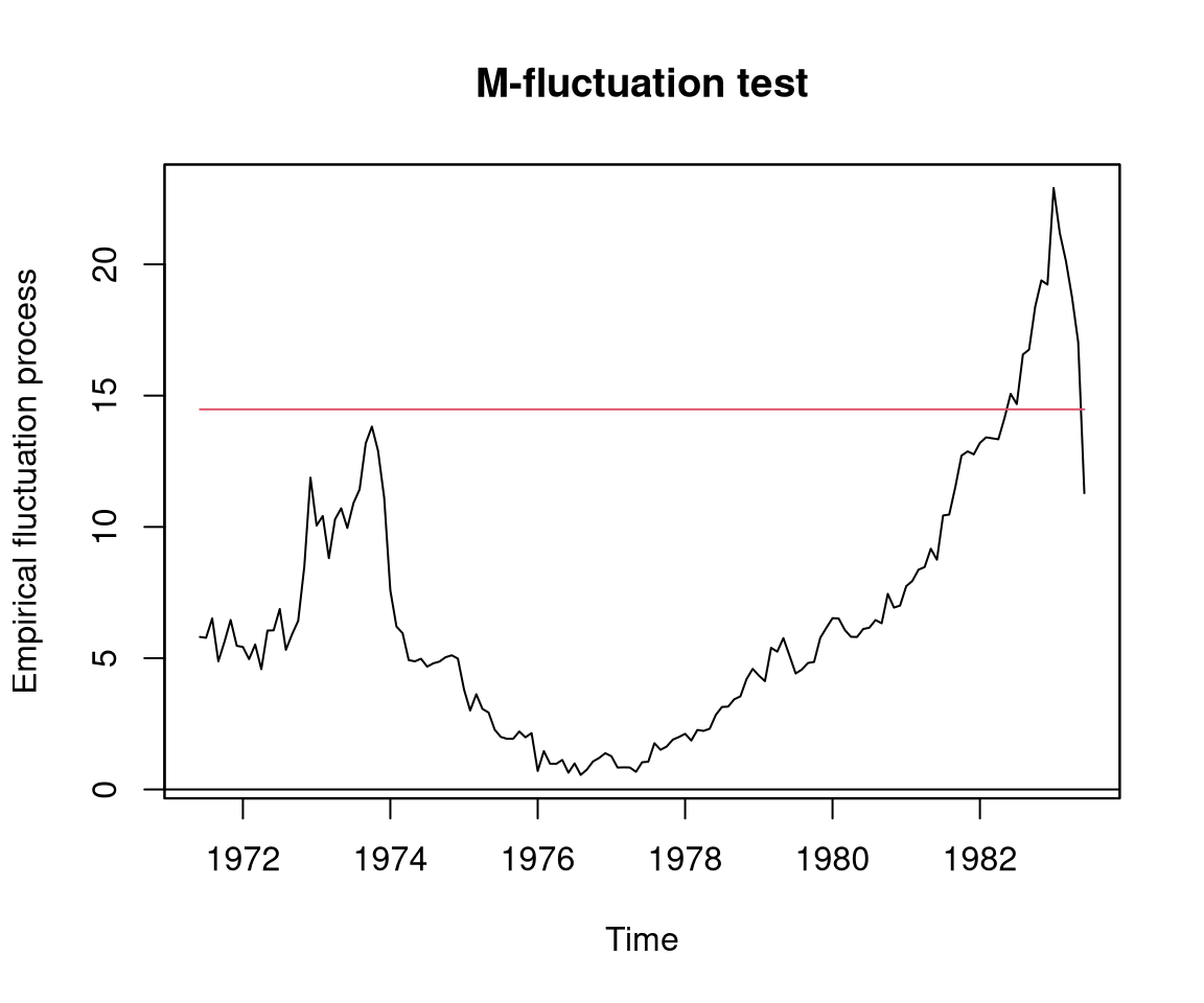
Rather than using the three separate commands above, it is also possible to carry out exactly the same test withe sample visualization in a single command:
The big advantage of the gefp() function is that it can not only be applied to lm() objects but to numerous other classes of models. Moreover, it facilitates assessment of parameter stability not just across time but across any available continuous, ordinal, or categorical variable (such as age, education level, or gender).
Dating breaks
As all of the families of tests considered in the sections above, show some significant changes in the parameters, a natural next step is the dating of these changes. This tries to answer the following questions.
Given that there is evidence for a structural change in \(i = 1, \dots, n\), it might be possible that stable regression relationships can be found on subsets of the data.
How many segments are in the data? Where are the breakpoints?
To answer these questions, the breakpoints() function from strucchange minimizes the residual sum of squares across all possible combinations of breakpoints. Internally, this employs a so-called dynamic programming algorithm (exploiting recursive residuals).
Subsequently, the plot(), summary(), and AIC() methods can help to select the final number of breakpoints to consider. Numerous other methods are available to extract further quantities of interest such as confidence intervals, fitted values and residuals, the segment-specific regression coefficients etc.
For the seatbelt data all combinations of breakpoints (while assuring a minimal segment size of 10% of the sample) can be computed and summarized as follows.
bp <- breakpoints(y ~ ylag1 + ylag12, data = seatbelt, h = 0.1)
summary(bp)
##
##   Optimal (m+1)-segment partition:
##
## Call:
## breakpoints.formula(formula = y ~ ylag1 + ylag12, h = 0.1, data = seatbelt)
##
## Breakpoints at observation number:
##
## m = 1      46
## m = 2      46                   157
## m = 3      46 70                157
## m = 4      46 70    108         157
## m = 5      46 70        120 141 160
## m = 6      46 70 89 108     141 160
## m = 7      46 70 89 107 125 144 162
## m = 8   18 46 70 89 107 125 144 162
##
## Corresponding to breakdates:
##
## m = 1           1973(10)
## m = 2           1973(10)                                             1983(1)
## m = 3           1973(10) 1975(10)                                    1983(1)
## m = 4           1973(10) 1975(10)         1978(12)                   1983(1)
## m = 5           1973(10) 1975(10)                  1979(12) 1981(9)  1983(4)
## m = 6           1973(10) 1975(10) 1977(5) 1978(12)          1981(9)  1983(4)
## m = 7           1973(10) 1975(10) 1977(5) 1978(11) 1980(5)  1981(12) 1983(6)
## m = 8   1971(6) 1973(10) 1975(10) 1977(5) 1978(11) 1980(5)  1981(12) 1983(6)
##
## Fit:
##
## m   0       1       2       3       4       5       6       7       8
## RSS    0.33    0.30    0.27    0.24    0.24    0.23    0.23    0.22    0.22
## BIC -602.86 -601.05 -598.90 -594.88 -577.29 -562.49 -546.36 -526.73 -506.99
plot(bp)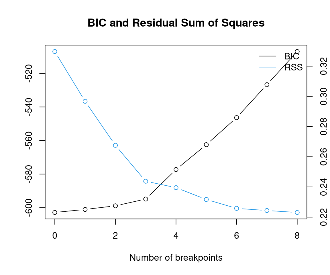
By default the breakpoints stored in bp correspond to the minimum BIC segmentation. Unfortunately, here the minimum BIC is attained for \(0\) breakpoints even though all of the tests above clearly rejected the null hypothesis of parameter stability. Bai and Perron (2003) report that the BIC has problems in dynamic regressions with lagged regressors. Therefore, due to the shape of the RE process of the \(F\) statistics, a model with two breakpoints is adopted here. Note also that this corresponds to the “elbow” in the residual sum of squares shown in the plot above.
The breakpoints and corresponding dates along with 95% confidence intervals for the two breaks are:
confint(bp, breaks = 2)
##
##   Confidence intervals for breakpoints
##   of optimal 3-segment partition:
##
## Call:
## confint.breakpointsfull(object = bp, breaks = 2)
##
## Breakpoints at observation number:
##   2.5 % breakpoints 97.5 %
## 1    33          46     56
## 2   144         157    171
##
## Corresponding to breakdates:
##   2.5 %    breakpoints 97.5 %
## 1 1972(9)  1973(10)    1974(8)
## 2 1981(12) 1983(1)     1984(3)
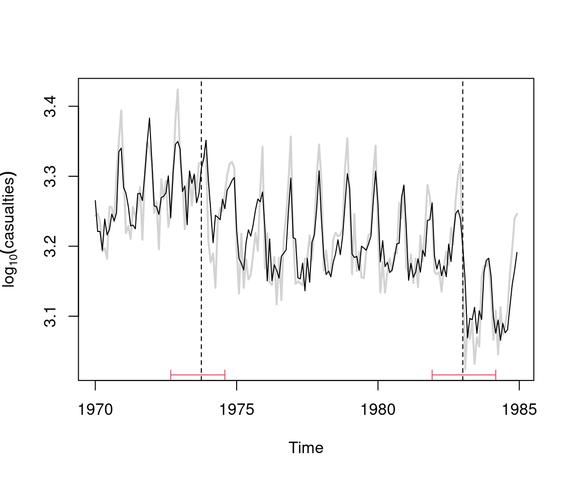
Note that these accurately match the oil crisis in October 1973 and the introduction of compulsary wearing of seatbelts in January 1983.
The corresponding regression coefficients on the three segments can be extracted as follows. These show that the seasonal autocorrelation went down over time while the non-seasonal autocorrelation at lag 1 went up.
coef(bp, breaks = 2)
##                    (Intercept)  ylag1 ylag12
## 1970(1) - 1973(10)      0.6331 0.1173 0.6945
## 1973(11) - 1983(1)      0.6663 0.2182 0.5723
## 1983(2) - 1984(12)      0.7326 0.5486 0.2142
The original time series along with the segmented fitted values and the confidence intervals for the breakpoints are visualized below. This suggests that the shifts in the series are captured resonably well.
Monitoring
Finally, fluctuation tests can be applied sequentially to monitor the stability of models while new observations are arriving in real time. Thus, monitoring aims to answer the following questions.
Given that a stable model could be established for \(n\) observations, the question is whether it remains stable in the future or:
Are incoming observations for \(i > n\) still consistent with the established model or do the parameters change?
More formally, this means that a sequential test of the null hypothesis
\[ H_0:~ \beta_i = \beta_0 \qquad (i > n) \]
is carried out against the alternative that \(\beta_i\) changes at some time in the future \(i > n\).
The basic assumption for this to work is that the model parameters are stab e \(\beta_i = \beta_0\) in the “history period” \(i = 1, \dots, n\).
In strucchange, the function mefp() initializes a monitoring fluctuation process wich can again be based on CUSUMs of different kinds of residuals or parameter estimates. Using the monitor() function the fluctuation process is updated as new data becomes available. Results can be inspected by print() or plot() methods.
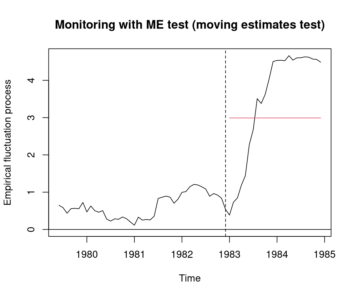
To illustrate this with the seatbelt data, monitoring is initialized for the time window from January 1976 to December 1982 (i.e., \(n = 84\) months). For this history period a stable SARIMA model can be estimated using least squares. Subsequently, the stability of the model is monitored starting from January 1983 when the seatbelt legislation changed in the UK. Here, a moving estimates (ME) process is used with a bandwidth of 50% of the history sample, i.e., a rolling window of \(42\) months.
The code chunk below makes all data after December 1982 available in one go. The ME process quickly deviates from zero, signaling a change in the parameters. It turns significant by crosses the border of critical values later in 1983.
References
Bai, Jushan, and Pierre Perron. 2003. “Computation and Analysis of Multiple Structural Change Models.” Journal of Applied Econometrics 18: 1–22. https://doi.org/10.1002/jae.659.
Harvey, A. C., and J. Durbin. 1986. “The Effects of Seat Belt Legislation on British Road Casualties: A Case Study in Structural Time Series Modelling.” Journal of the Royal Statistical Society A 149 (3): 187–227. https://doi.org/10.2307/2981553.
Merkle, Edgar C., and Achim Zeileis. 2013. “Tests of Measurement Invariance Without Subgroups: A Generalization of Classical Methods.” Psychometrika 78 (1): 59–82. https://doi.org/10.1007/s11336-012-9302-4.
Zeileis, Achim. 2005. “A Unified Approach to Structural Change Tests Based on ML Scores, \(F\) Statistics, and OLS Residuals.” Econometric Reviews 24 (4): 445–66. https://doi.org/10.1080/07474930500406053.
Zeileis, Achim. 2006. “Implementing a Class of Structural Change Tests: An Econometric Computing Approach.” Computational Statistics & Data Analysis 50: 2987–3008. https://doi.org/10.1016/j.csda.2005.07.001.
Zeileis, Achim, and Gabor Grothendieck. 2005. “zoo: S3 Infrastructure for Regular and Irregular Time Series.” Journal of Statistical Software 14 (6): 1–27. https://doi.org/10.18637/jss.v014.i06.
Zeileis, Achim, and Kurt Hornik. 2007. “Generalized M-Fluctuation Tests for Parameter Instability.” Statistica Neerlandica 61 (4): 488–508. https://doi.org/10.1111/j.1467-9574.2007.00371.x.
Zeileis, Achim, Torsten Hothorn, and Kurt Hornik. 2008. “Model-Based Recursive Partitioning.” Journal of Computational and Graphical Statistics 17 (2): 492–514. https://doi.org/10.1198/106186008X319331.
Zeileis, Achim, Christian Kleiber, Walter Krämer, and Kurt Hornik. 2003. “Testing and Dating of Structural Changes in Practice.” Computational Statistics & Data Analysis 44 (1–2): 109–23. https://doi.org/10.1016/S0167-9473(03)00030-6.
Zeileis, Achim, Friedrich Leisch, Kurt Hornik, and Christian Kleiber. 2002. “strucchange: An R Package for Testing for Structural Change in Linear Regression Models.” Journal of Statistical Software 7 (2): 1–38. https://doi.org/10.18637/jss.v007.i02.