German M1 Money Demand

Description

German M1 money demand.

Usage

data("GermanM1")

Format

GermanM1 is a data frame containing 12 quarterly time series from 1961(1) to 1995(4) and two further variables. historyM1 is the subset of GermanM1 up to 1990(2), i.e., the data before the German monetary unification on 1990-06-01. monitorM1 is the complement of historyM1, i.e., the data after the unification. All three data frames contain the variables

m

time series. Logarithm of real M1 per capita,

p

time series. Logarithm of a price index,

y

time series. Logarithm of real per capita gross national product,

R

time series. Long-run interest rate,

dm

time series. First differences of m,

dy2

time series. First differences of lag 2 of y,

dR

time series. First differences of R,

dR1

time series. First differences of lag 1 of R,

dp

time series. First differences of p,

m1

time series. Lag 1 of m,

y1

time series. Lag 1 of y,

R1

time series. Lag 1 of R,

season

factor coding the seasonality,

ecm.res

vector containing the OLS residuals of the Lütkepohl et al. (1999) model fitted in the history period.

Details

Lütkepohl et al. (1999) investigate the linearity and stability of German M1 money demand: they find a stable regression relation for the time before the monetary union on 1990-06-01 but a clear structural instability afterwards.

Zeileis et al. (2005) use a model with ecm.res instead of m1, y1 and R1, which leads to equivalent results in the history period but slightly different results in the monitoring period. The reason for the replacement is that stationary regressors are needed for the structural change tests. See references and the examples below for more details.

Source

The data is provided by the German central bank and is available online in the data archive of the Journal of Applied Econometrics http://qed.econ.queensu.ca/jae/1999-v14.5/lutkepohl-terasvirta-wolters/.

References

Lütkepohl H., Teräsvirta T., Wolters J. (1999), Investigating Stability and Linearity of a German M1 Money Demand Function, Journal of Applied Econometrics, 14, 511-525.

Zeileis A., Leisch F., Kleiber C., Hornik K. (2005), Monitoring Structural Change in Dynamic Econometric Models, Journal of Applied Econometrics, 20, 99–121.

Examples

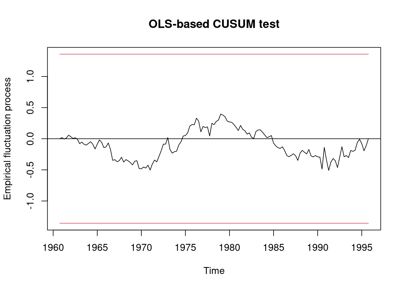
library("strucchange")

data("GermanM1")
## Lütkepohl et al. (1999) use the following model
LTW.model <- dm ~ dy2 + dR + dR1 + dp + m1 + y1 + R1 + season
## Zeileis et al. (2005) use
M1.model <- dm ~ dy2 + dR + dR1 + dp + ecm.res + season


## historical tests
ols <- efp(LTW.model, data = GermanM1, type = "OLS-CUSUM")
plot(ols)

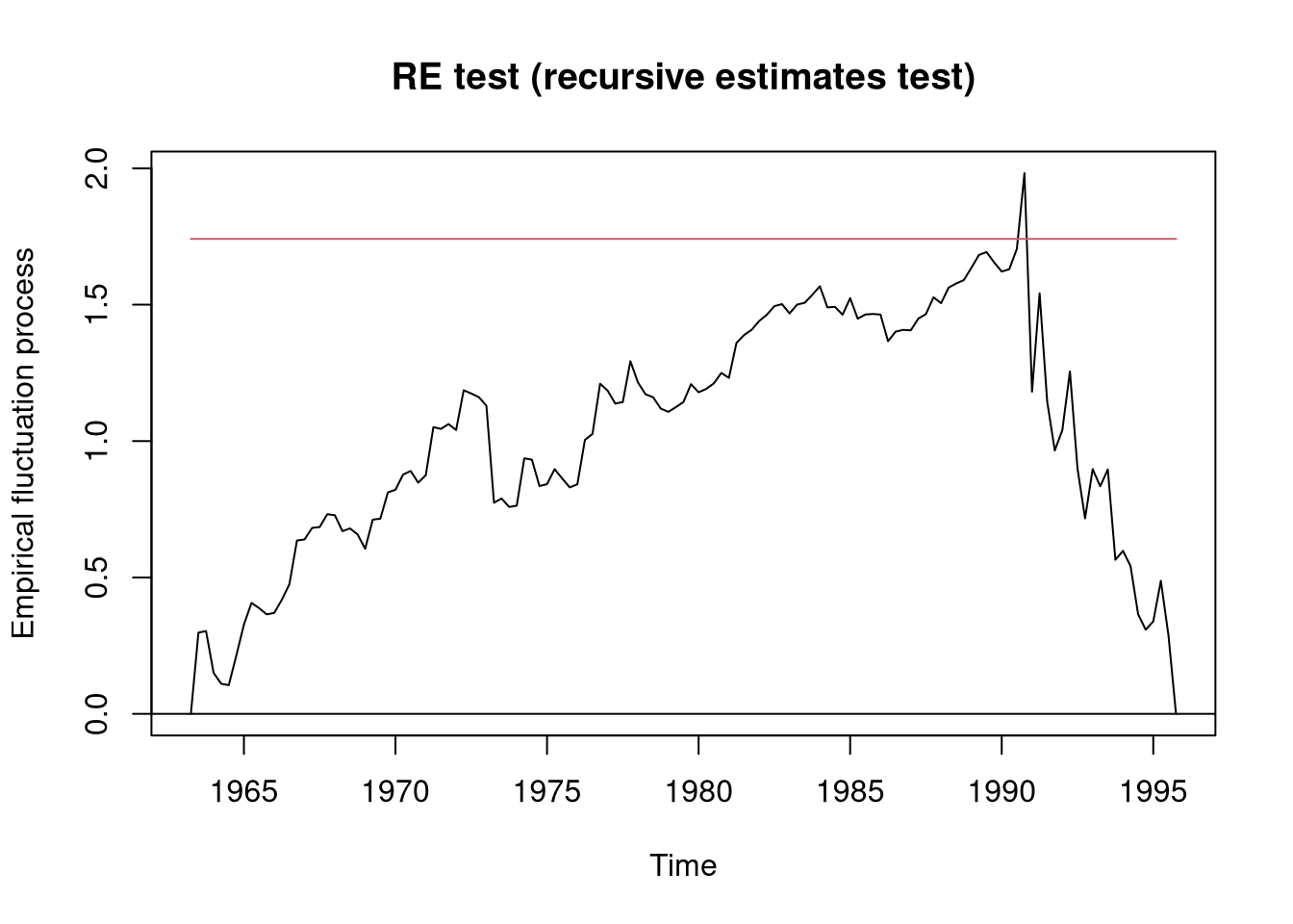
re <- efp(LTW.model, data = GermanM1, type = "fluctuation")
plot(re)

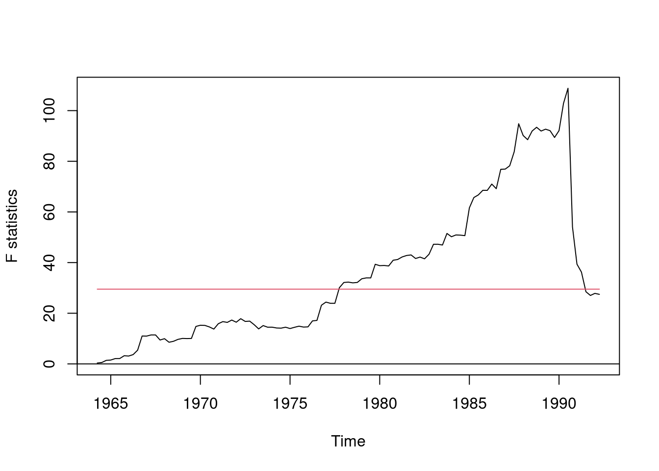
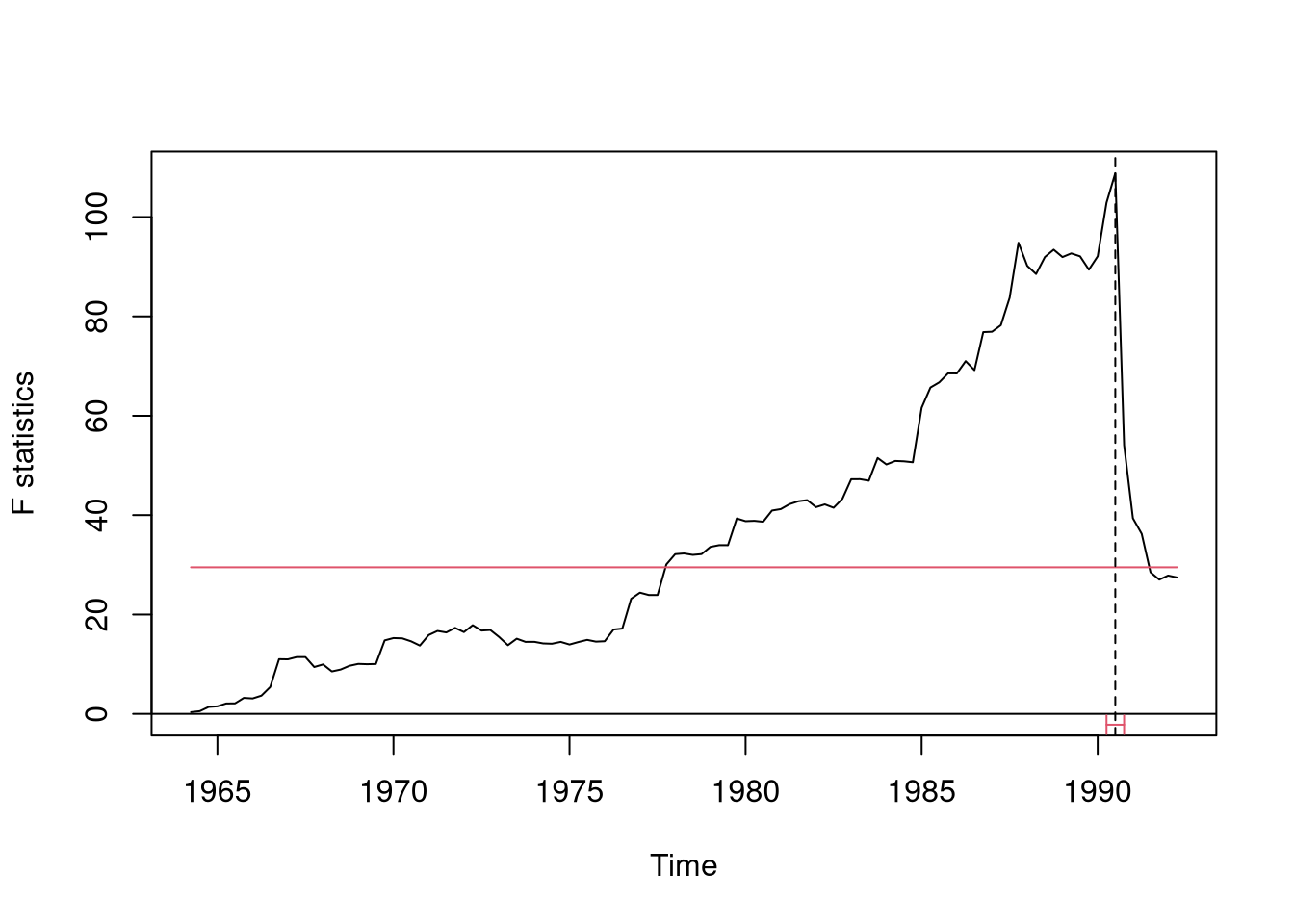
fs <- Fstats(LTW.model, data = GermanM1, from = 0.1)
plot(fs)

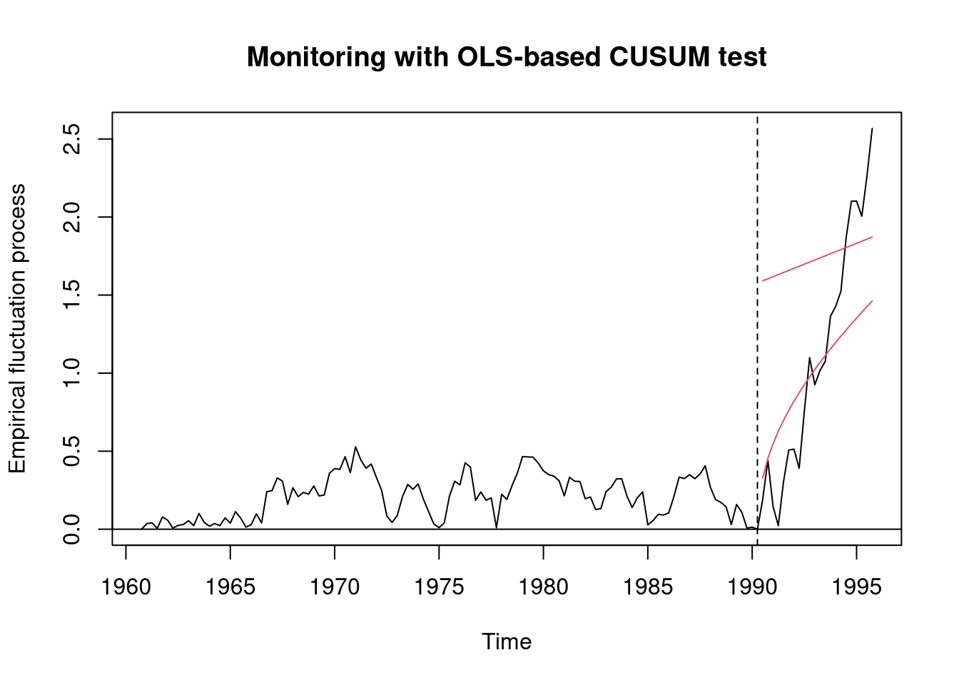
## monitoring
M1 <- historyM1
ols.efp <- efp(M1.model, type = "OLS-CUSUM", data = M1)
newborder <- function(k) 1.5778*k/118
ols.mefp <- mefp(ols.efp, period = 2)
ols.mefp2 <- mefp(ols.efp, border = newborder)
M1 <- GermanM1
ols.mon <- monitor(ols.mefp)

Break detected at observation # 128 

ols.mon2 <- monitor(ols.mefp2)

Break detected at observation # 135 

plot(ols.mon)
lines(boundary(ols.mon2), col = 2)

## dating
bp <- breakpoints(LTW.model, data = GermanM1)
summary(bp)

     Optimal (m+1)-segment partition: 

Call:
breakpoints.formula(formula = LTW.model, data = GermanM1)

Breakpoints at observation number:
                       
m = 1               119
m = 2      42       119
m = 3      48 71    119
m = 4   27 48 71    119
m = 5   27 48 71 98 119

Corresponding to breakdates:
                                               
m = 1                                   1990(3)
m = 2           1971(2)                 1990(3)
m = 3           1972(4) 1978(3)         1990(3)
m = 4   1967(3) 1972(4) 1978(3)         1990(3)
m = 5   1967(3) 1972(4) 1978(3) 1985(2) 1990(3)

Fit:
                                                                     
m   0          1          2          3          4          5         
RSS  3.683e-02  1.916e-02  1.522e-02  1.301e-02  1.053e-02  9.198e-03
BIC -6.974e+02 -7.296e+02 -7.025e+02 -6.653e+02 -6.356e+02 -5.952e+02

plot(bp)

plot(fs)
lines(confint(bp))