Computes a series of F statistics for a specified data window.
Usage
Fstats(formula, from = 0.15, to = NULL, data = list(), vcov. = NULL)
Arguments
formula
a symbolic description for the model to be tested
from, to
numeric. If from is smaller than 1 they are interpreted as percentages of data and by default to is taken to be 1 - from. F statistics will be calculated for the observations (nfrom):(nto), when n is the number of observations in the model. If from is greater than 1 it is interpreted to be the index and to defaults to n - from. If from is a vector with two elements, then from and to are interpreted as time specifications like in ts, see also the examples.
data
an optional data frame containing the variables in the model. By default the variables are taken from the environment which Fstats is called from.
vcov.
a function to extract the covariance matrix for the coefficients of a fitted model of class “lm”.
Details
For every potential change point in from:to a F statistic (Chow test statistic) is computed. For this an OLS model is fitted for the observations before and after the potential change point, i.e. 2k parameters have to be estimated, and the error sum of squares is computed (ESS). Another OLS model for all observations with a restricted sum of squares (RSS) is computed, hence k parameters have to be estimated here. If n is the number of observations and k the number of regressors in the model, the formula is:
\(F = \frac{(RSS - ESS)}{ESS/(n - 2 k)}\)
Note that this statistic has an asymptotic chi-squared distribution with k degrees of freedom and (under the assumption of normality) F/k has an exact F distribution with k and n - 2k degrees of freedom.
Value
Fstats returns an object of class “Fstats”, which contains mainly a time series of F statistics. The function plot has a method to plot the F statistics or the corresponding p values; with sctest a supF-, aveF- or expF-test on structural change can be performed.
References
Andrews D.W.K. (1993), Tests for parameter instability and structural change with unknown change point, Econometrica, 61, 821-856.
Hansen B. (1992), Tests for parameter instability in regressions with I(1) processes, Journal of Business & Economic Statistics, 10, 321-335.
Hansen B. (1997), Approximate asymptotic p values for structural-change tests, Journal of Business & Economic Statistics, 15, 60-67.
See Also
plot.Fstats, sctest.Fstats, boundary.Fstats
Examples
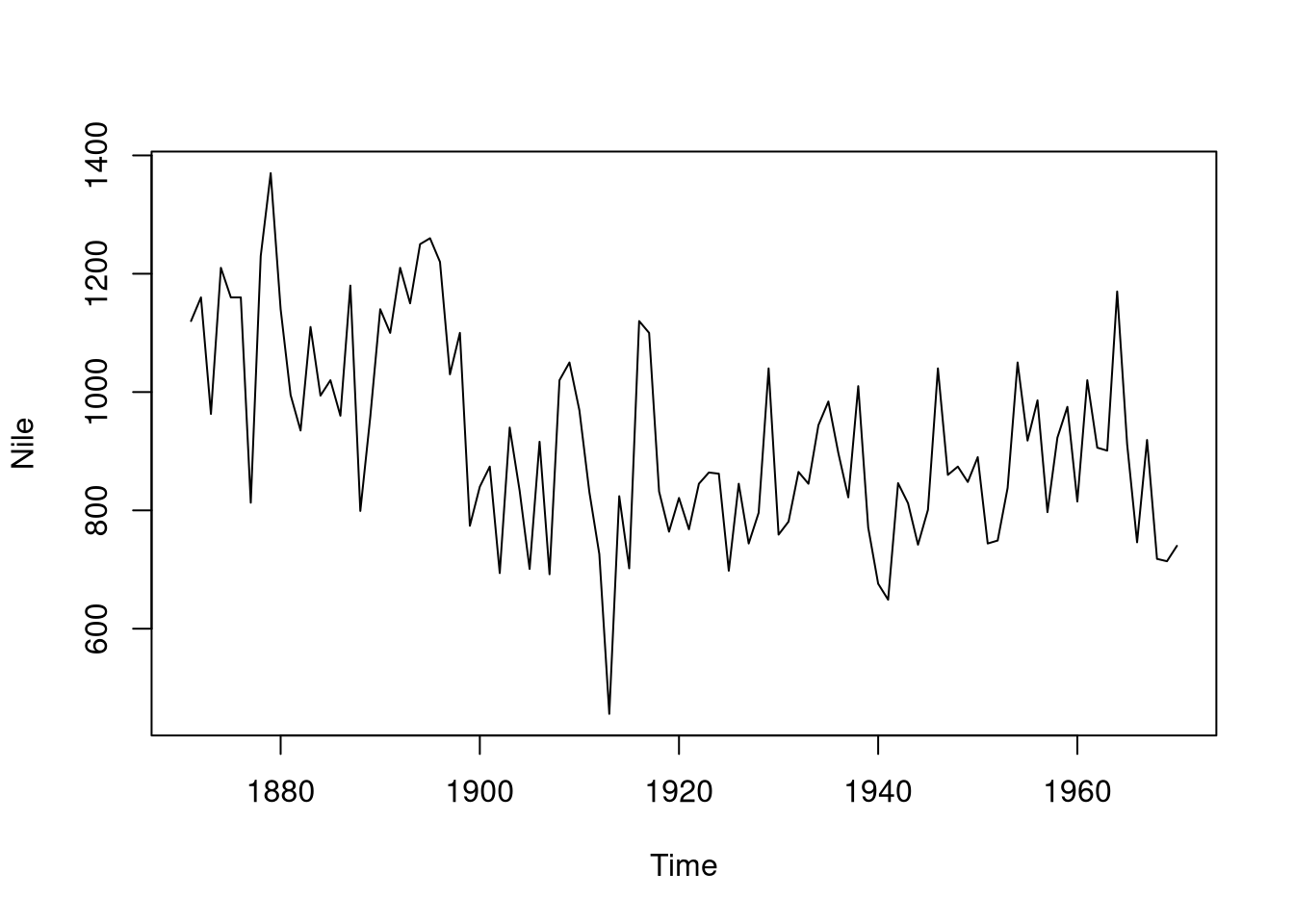
library("strucchange")## Nile data with one breakpoint: the annual flows drop in 1898## because the first Ashwan dam was builtdata("Nile")plot(Nile)
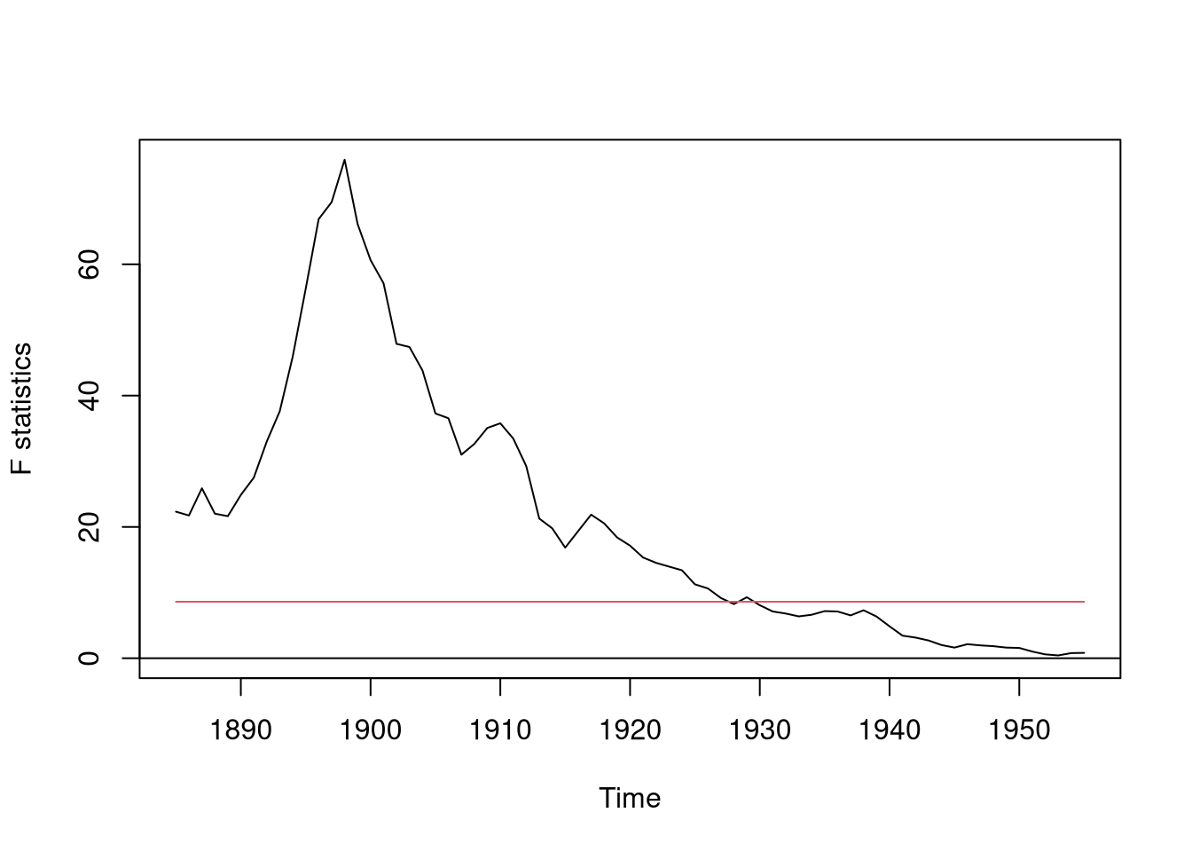
## test the null hypothesis that the annual flow remains constant## over the yearsfs.nile<-Fstats(Nile~1)plot(fs.nile)
    supF test

data:  fs.nile
sup.F = 75.93, p-value = 2.22e-16
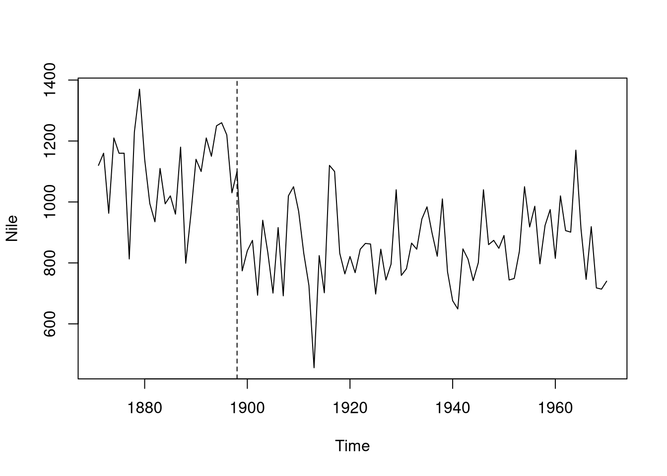
## visualize the breakpoint implied by the argmax of the F statisticsplot(Nile)lines(breakpoints(fs.nile))
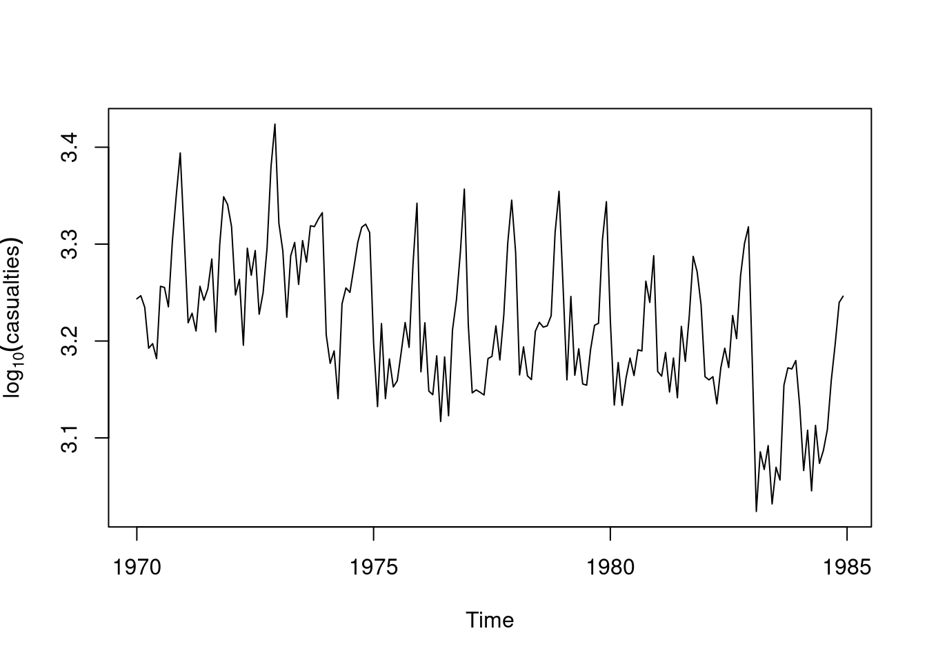
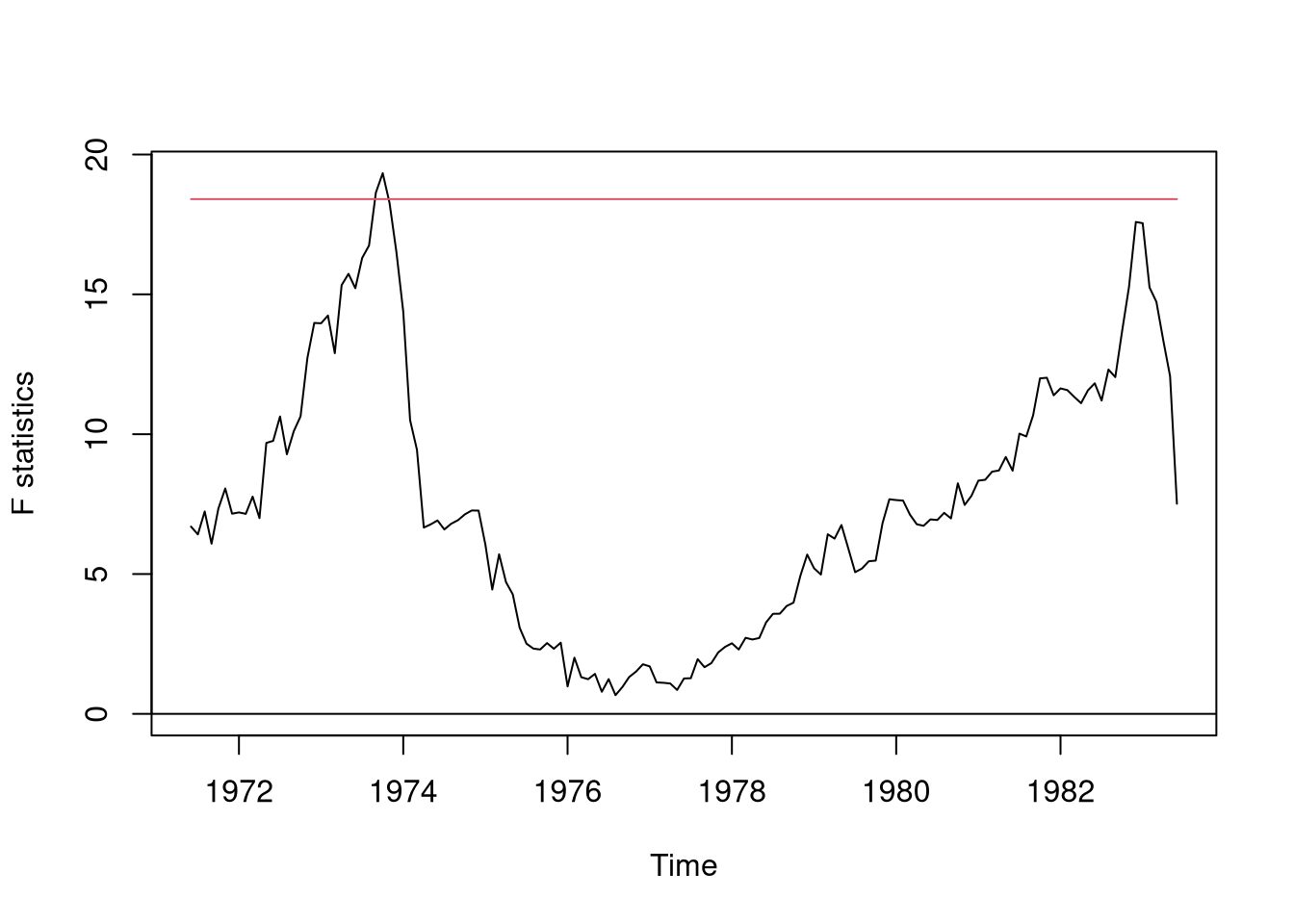
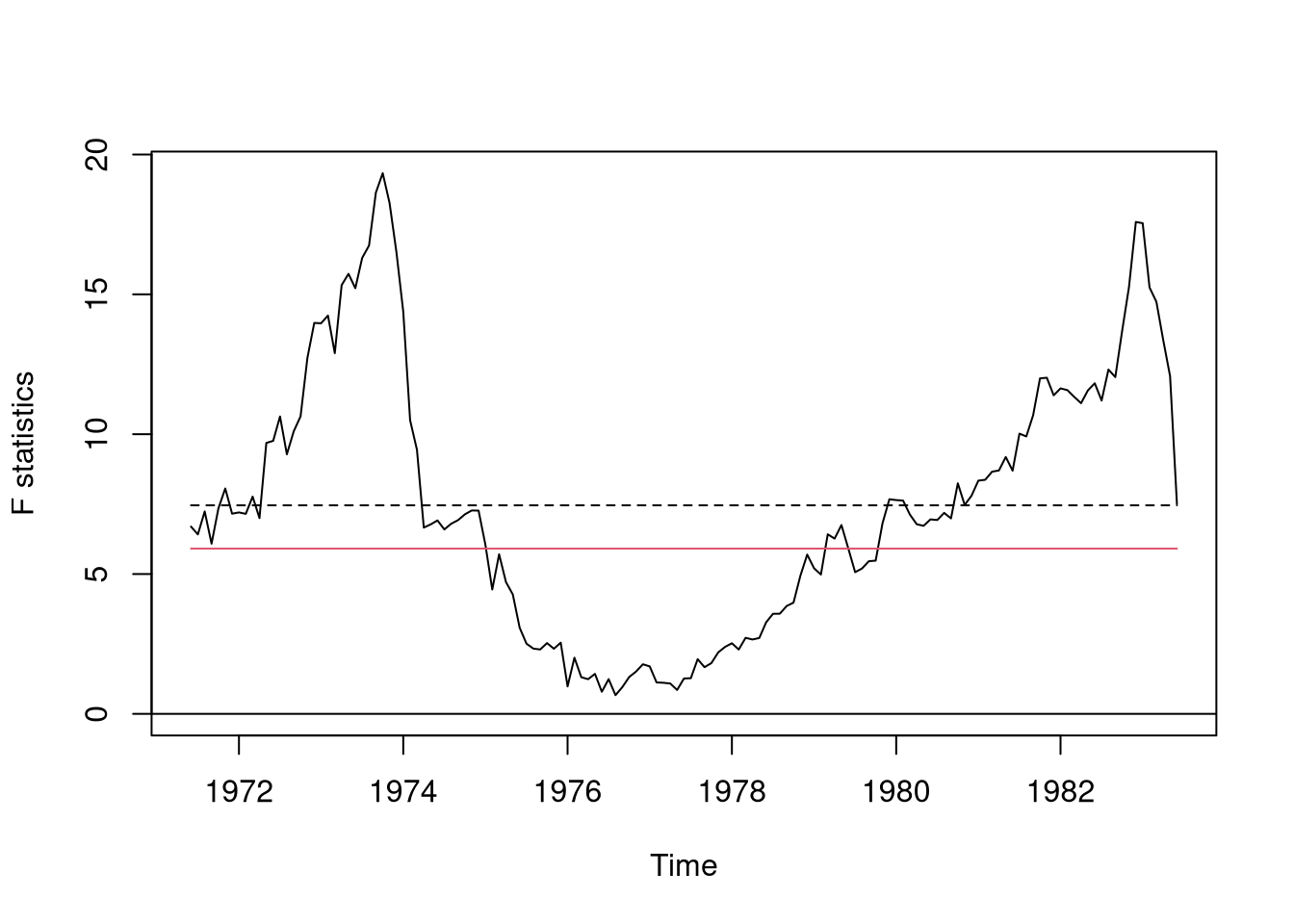
## UK Seatbelt data: a SARIMA(1,0,0)(1,0,0)_12 model## (fitted by OLS) is used and reveals (at least) two## breakpoints - one in 1973 associated with the oil crisis and## one in 1983 due to the introduction of compulsory## wearing of seatbelts in the UK.data("UKDriverDeaths")seatbelt<-log10(UKDriverDeaths)seatbelt<-cbind(seatbelt, lag(seatbelt, k =-1), lag(seatbelt, k =-12))colnames(seatbelt)<-c("y", "ylag1", "ylag12")seatbelt<-window(seatbelt, start =c(1970, 1), end =c(1984,12))plot(seatbelt[,"y"], ylab =expression(log[10](casualties)))
## compute F statistics for potential breakpoints between## 1971(6) (corresponds to from = 0.1) and 1983(6) (corresponds to## to = 0.9 = 1 - from, the default)## compute F statisticsfs<-Fstats(y~ylag1+ylag12, data =seatbelt, from =0.1)## this gives the same resultfs<-Fstats(y~ylag1+ylag12, data =seatbelt, from =c(1971, 6), to =c(1983, 6))## plot the F statisticsplot(fs, alpha =0.01)
## plot F statistics with aveF boundaryplot(fs, aveF =TRUE)