strucchange

Marriages, Births and Deaths in Grossarl

Description

Data about the number of marriages, illegitimate and legitimate births, and deaths in the Austrian Alpine village Grossarl during the 18th and 19th century.

Usage

data("Grossarl")

Format

Grossarl is a data frame containing 6 annual time series (1700 - 1899), 3 factors coding policy interventions and 1 vector with the year (plain numeric).

marriages: time series. Number of marriages,
illegitimate: time series. Number of illegitimate births,
legitimate: time series. Number of legitimate births,
legitimate: time series. Number of deaths,
fraction: time series. Fraction of illegitimate births,
lag.marriages: time series. Number of marriages in the previous year,
politics: ordered factor coding 4 different political regimes,
morals: ordered factor coding 5 different moral regulations,
nuptiality: ordered factor coding 5 different marriage restrictions,
year: numeric. Year of observation.

Details

The data frame contains historical demographic data from Grossarl, a village in the Alpine region of Salzburg, Austria, during the 18th and 19th century. During this period, the total population of Grossarl did not vary much on the whole, with the very exception of the period of the protestant emigrations in 1731/32.

Especially during the archbishopric, moral interventions aimed at lowering the proportion of illegitimate baptisms. For details see the references.

Source

Parish registers provide the basic demographic series of baptisms and burials (which is almost equivalent to births and deaths in the study area) and marriages. For more information see Veichtlbauer et al. (2006).

References

Veichtlbauer O., Zeileis A., Leisch F. (2006), The Impact Of Policy Interventions on a Pre-Industrial Population System in the Austrian Alps, forthcoming.

Zeileis A., Veichtlbauer O. (2002), Policy Interventions Affecting Illegitimacy in Preindustrial Austria: A Structural Change Analysis, In R. Dutter (ed.), Festschrift 50 Jahre Österreichische Statistische Gesellschaft, 133-146, Österreichische Statistische Gesellschaft.

Examples

library("strucchange")

data("Grossarl")

## time series of births, deaths, marriages
###########################################

with(Grossarl, plot(cbind(deaths, illegitimate + legitimate, marriages),
  plot.type = "single", col = grey(c(0.7, 0, 0)), lty = c(1, 1, 3),
  lwd = 1.5, ylab = "annual Grossarl series"))
legend("topright", c("deaths", "births", "marriages"), col = grey(c(0.7, 0, 0)),
  lty = c(1, 1, 3), bty = "n")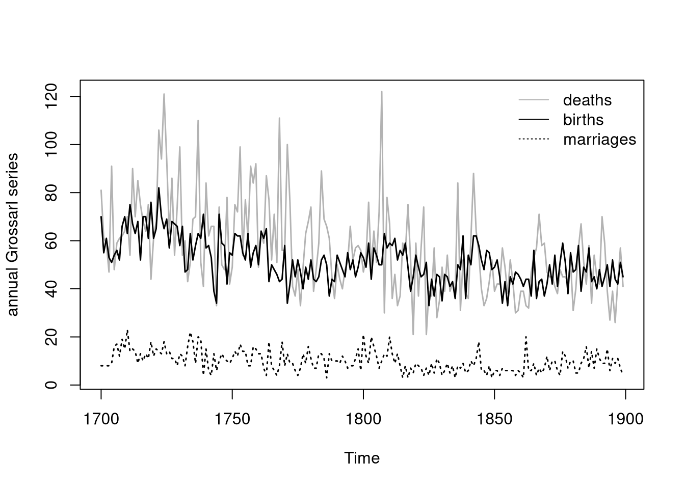

## illegitimate births
######################
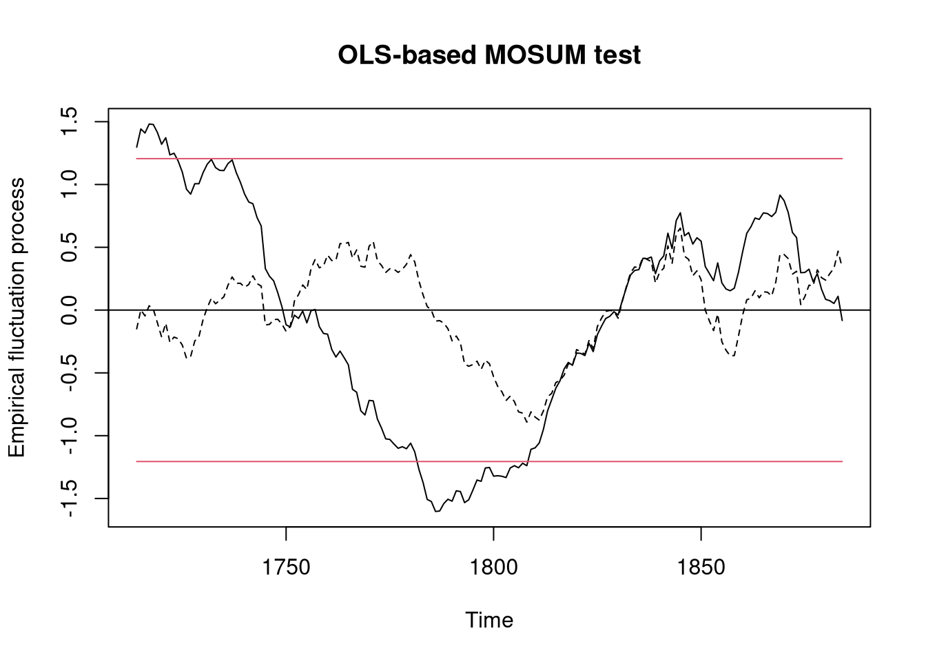
## lm + MOSUM
plot(Grossarl$fraction)
fm.min <- lm(fraction ~ politics, data = Grossarl)
fm.ext <- lm(fraction ~ politics + morals + nuptiality + marriages,
  data = Grossarl)
lines(ts(fitted(fm.min), start = 1700), col = 2)
lines(ts(fitted(fm.ext), start = 1700), col = 4)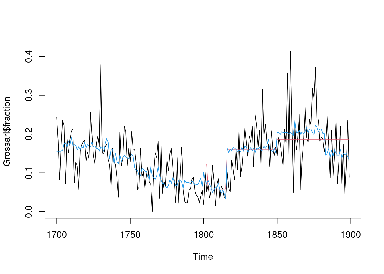

mos.min <- efp(fraction ~ politics, data = Grossarl, type = "OLS-MOSUM")
mos.ext <- efp(fraction ~ politics + morals + nuptiality + marriages,
  data = Grossarl, type = "OLS-MOSUM")
plot(mos.min)
lines(mos.ext, lty = 2)

## dating
bp <- breakpoints(fraction ~ 1, data = Grossarl, h = 0.1)
summary(bp)


     Optimal (m+1)-segment partition: 

Call:
breakpoints.formula(formula = fraction ~ 1, h = 0.1, data = Grossarl)

Breakpoints at observation number:
                                    
m = 1                127            
m = 2      55        122            
m = 3      55        124         180
m = 4      55        122     157 179
m = 5      54 86     122     157 179
m = 6   35 55 86     122     157 179
m = 7   35 55 80 101 122     157 179
m = 8   35 55 79 99  119 139 159 179

Corresponding to breakdates:
                                               
m = 1                       1826               
m = 2        1754           1821               
m = 3        1754           1823           1879
m = 4        1754           1821      1856 1878
m = 5        1753 1785      1821      1856 1878
m = 6   1734 1754 1785      1821      1856 1878
m = 7   1734 1754 1779 1800 1821      1856 1878
m = 8   1734 1754 1778 1798 1818 1838 1858 1878

Fit:
                                                                         
m   0         1         2         3         4         5         6        
RSS    1.1088    0.8756    0.6854    0.6587    0.6279    0.6019    0.5917
BIC -460.8402 -497.4625 -535.8459 -533.1857 -532.1789 -530.0501 -522.8510
                       
m   7         8        
RSS    0.5934    0.6084
BIC -511.7017 -496.0924

## RSS, BIC, AIC
plot(bp)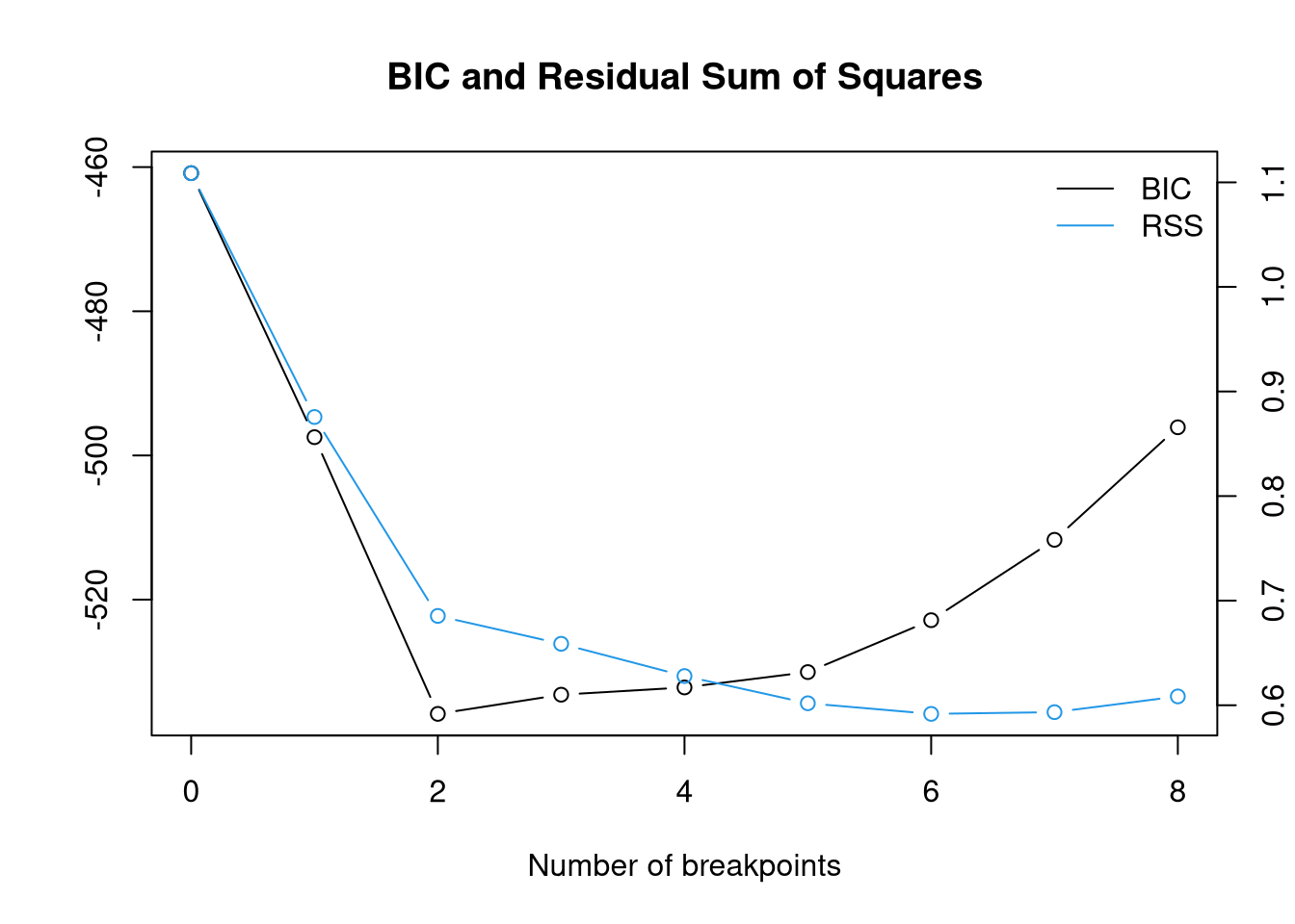

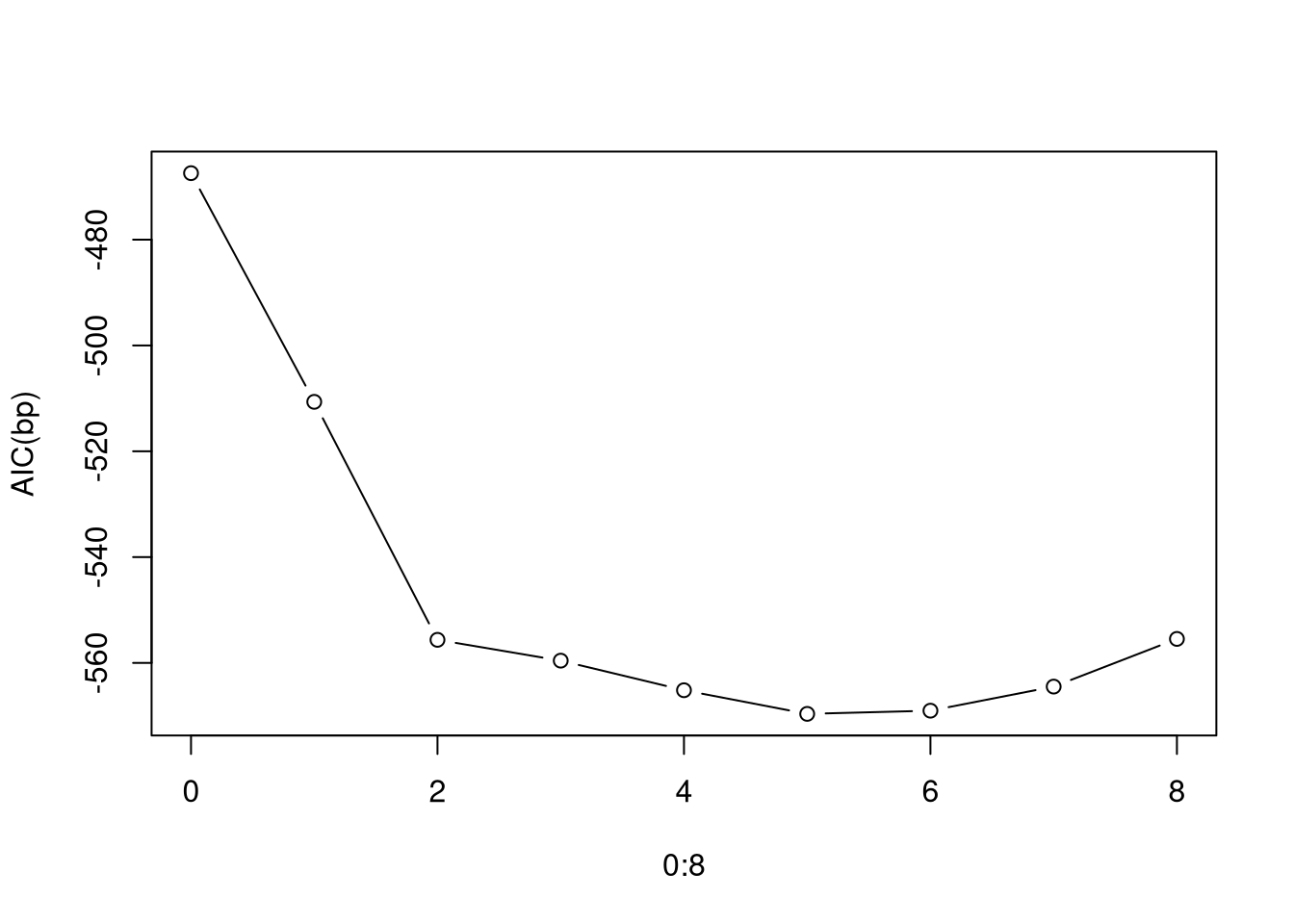
plot(0:8, AIC(bp), type = "b")

## probably use 5 or 6 breakpoints and compare with
## coding of the factors as used by us
##
## politics                   1803      1816 1850
## morals      1736 1753 1771 1803
## nuptiality                 1803 1810 1816      1883
##
## m = 5            1753 1785           1821 1856 1878
## m = 6       1734 1754 1785           1821 1856 1878
##              6    2    5              1    4    3

## fitted models
coef(bp, breaks = 6)

            (Intercept)
1700 - 1734  0.16933985
1735 - 1754  0.14078070
1755 - 1785  0.09890276
1786 - 1821  0.05955620
1822 - 1856  0.17441529
1857 - 1878  0.22425604
1879 - 1899  0.15414723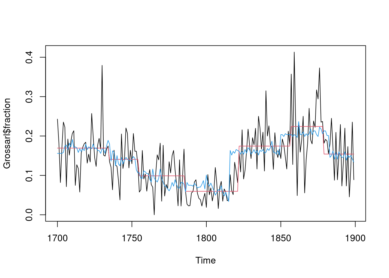

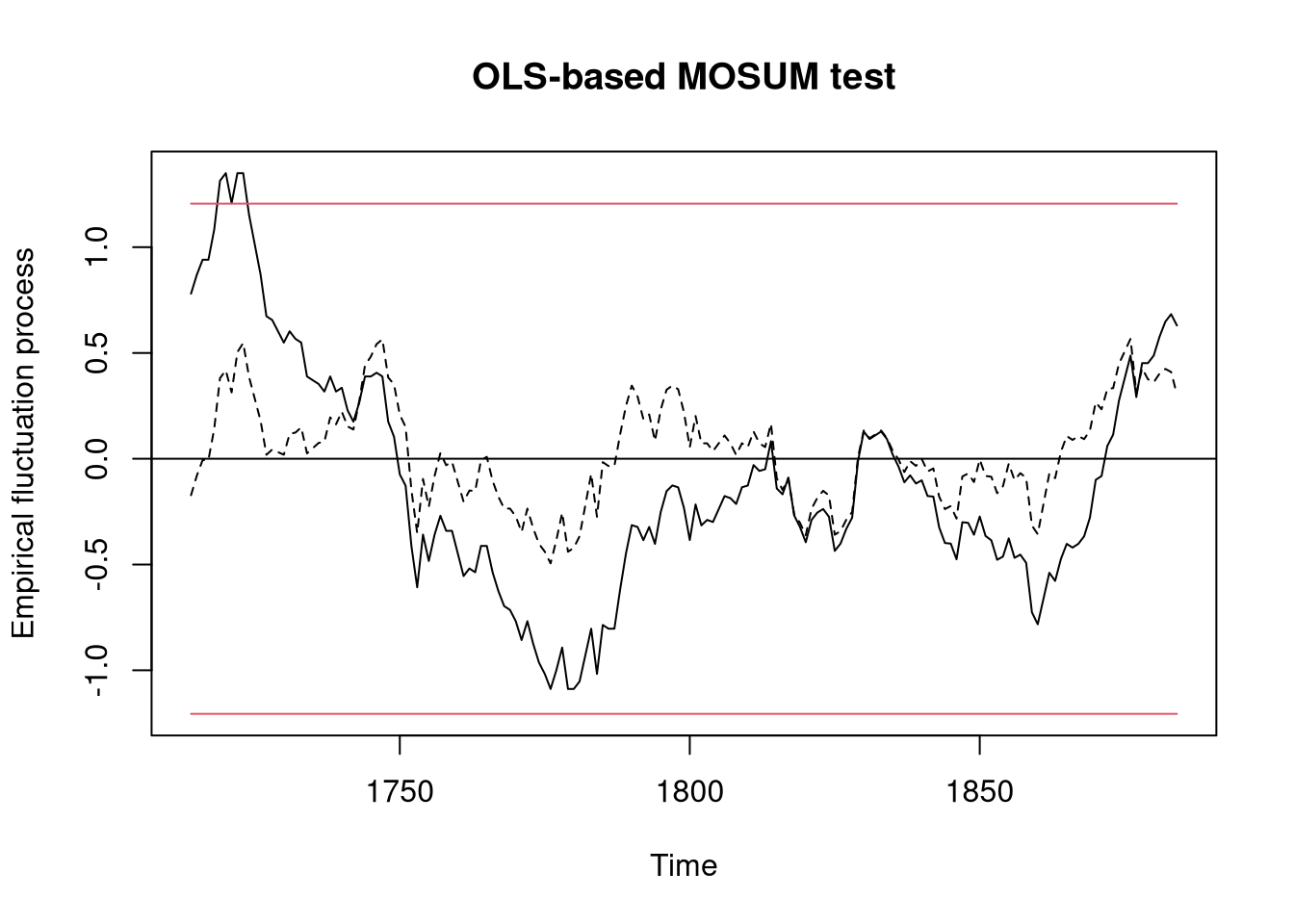
plot(Grossarl$fraction)
lines(fitted(bp, breaks = 6), col = 2)
lines(ts(fitted(fm.ext), start = 1700), col = 4)

## marriages
############
## lm + MOSUM
plot(Grossarl$marriages)
fm.min <- lm(marriages ~ politics, data = Grossarl)
fm.ext <- lm(marriages ~ politics + morals + nuptiality, data = Grossarl)
lines(ts(fitted(fm.min), start = 1700), col = 2)
lines(ts(fitted(fm.ext), start = 1700), col = 4)

mos.min <- efp(marriages ~ politics, data = Grossarl, type = "OLS-MOSUM")
mos.ext <- efp(marriages ~ politics + morals + nuptiality, data = Grossarl,
  type = "OLS-MOSUM")
plot(mos.min)
lines(mos.ext, lty = 2)

## dating
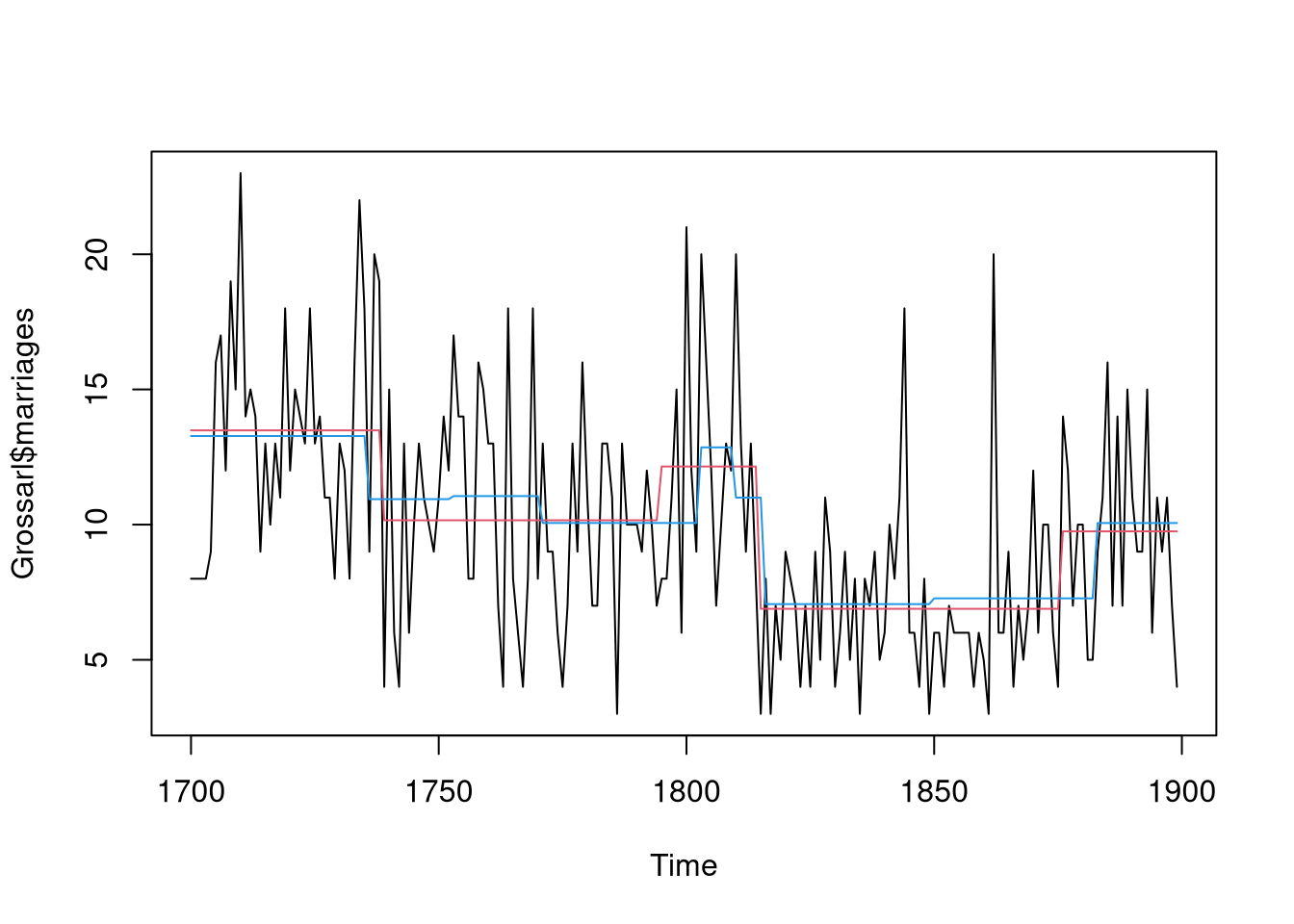
bp <- breakpoints(marriages ~ 1, data = Grossarl, h = 0.1)
summary(bp)


     Optimal (m+1)-segment partition: 

Call:
breakpoints.formula(formula = marriages ~ 1, h = 0.1, data = Grossarl)

Breakpoints at observation number:
                                   
m = 1               114            
m = 2      39       114            
m = 3      39       114         176
m = 4      39    95 115         176
m = 5      39 62 95 115         176
m = 6      39 62 95 115 136     176
m = 7      39 62 95 115 136 156 176
m = 8   21 41 62 95 115 136 156 176

Corresponding to breakdates:
                                               
m = 1                       1813               
m = 2        1738           1813               
m = 3        1738           1813           1875
m = 4        1738      1794 1814           1875
m = 5        1738 1761 1794 1814           1875
m = 6        1738 1761 1794 1814 1835      1875
m = 7        1738 1761 1794 1814 1835 1855 1875
m = 8   1720 1740 1761 1794 1814 1835 1855 1875

Fit:
                                                
m   0    1    2    3    4    5    6    7    8   
RSS 3832 3059 2863 2723 2671 2634 2626 2626 2645
BIC 1169 1134 1132 1132 1139 1147 1157 1167 1179

## RSS, BIC, AIC
plot(bp)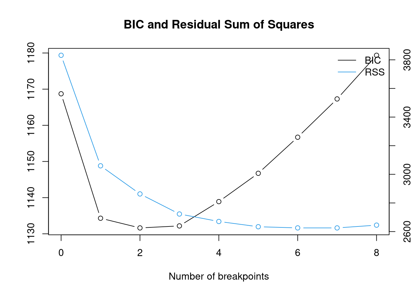

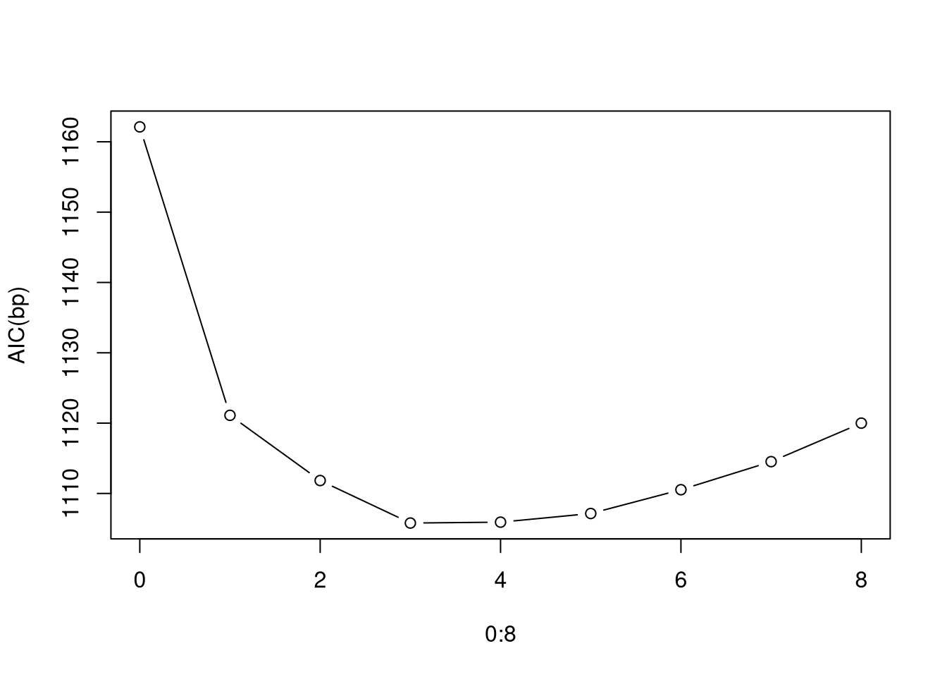
plot(0:8, AIC(bp), type = "b")

## probably use 3 or 4 breakpoints and compare with
## coding of the factors as used by us
##
## politics                   1803      1816 1850
## morals      1736 1753 1771 1803
## nuptiality                 1803 1810 1816      1883
##
## m = 3       1738                     1813      1875
## m = 4       1738      1794           1814      1875
##              2         4              1         3

## fitted models
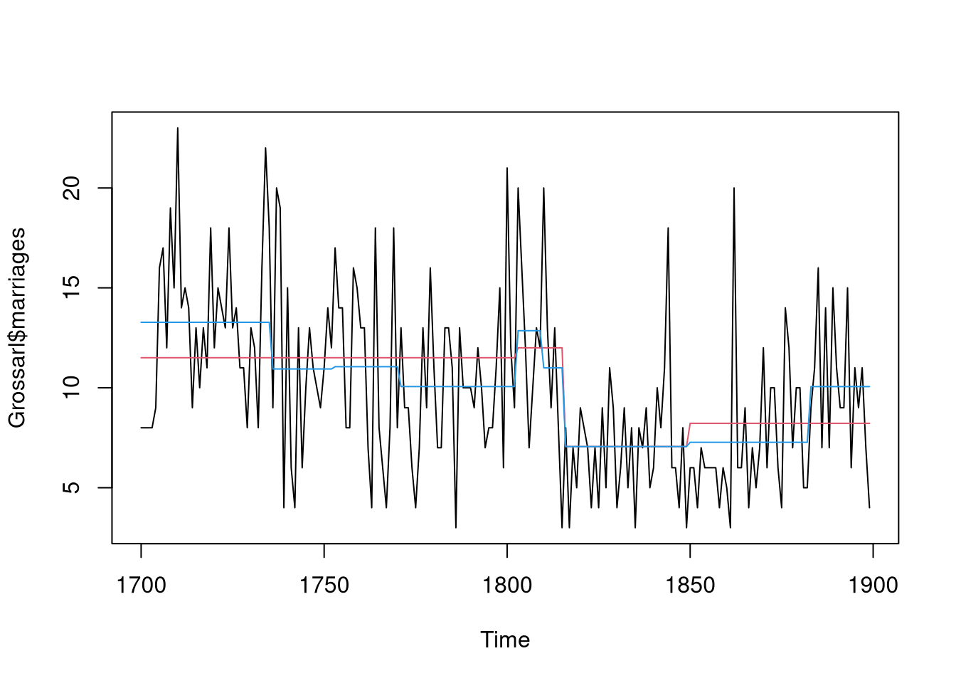
coef(bp, breaks = 4)

            (Intercept)
1700 - 1738   13.487179
1739 - 1794   10.160714
1795 - 1814   12.150000
1815 - 1875    6.885246
1876 - 1899    9.750000

plot(Grossarl$marriages)
lines(fitted(bp, breaks = 4), col = 2)
lines(ts(fitted(fm.ext), start = 1700), col = 4)