strucchange

UK Phillips Curve Equation Data

Description

Macroeconomic time series from the United Kingdom with variables for estimating the Phillips curve equation.

Usage

data("PhillipsCurve")

Format

A multivariate annual time series from 1857 to 1987 with the columns

p: Logarithm of the consumer price index,
w: Logarithm of nominal wages,
u: Unemployment rate,
dp: First differences of p,
dw: First differences of w,
du: First differences of u
u1: Lag 1 of u,
dp1: Lag 1 of dp.

Source

The data is available online in the data archive of the Journal of Applied Econometrics http://qed.econ.queensu.ca/jae/2003-v18.1/bai-perron/.

References

Alogoskoufis G.S., Smith R. (1991), The Phillips Curve, the Persistence of Inflation, and the Lucas Critique: Evidence from Exchange Rate Regimes, American Economic Review, 81, 1254-1275.

Bai J., Perron P. (2003), Computation and Analysis of Multiple Structural Change Models, Journal of Applied Econometrics, 18, 1-22.

Examples

library("strucchange")

## load and plot data
data("PhillipsCurve")
uk <- window(PhillipsCurve, start = 1948)
plot(uk[, "dp"])

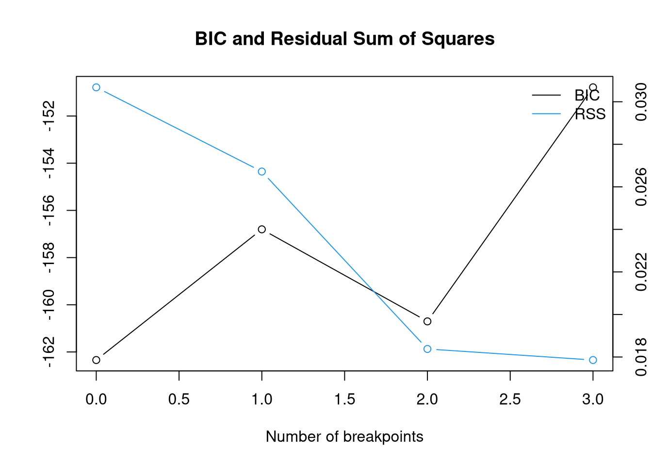
## AR(1) inflation model
## estimate breakpoints
bp.inf <- breakpoints(dp ~ dp1, data = uk, h = 8)
plot(bp.inf)

summary(bp.inf)


     Optimal (m+1)-segment partition: 

Call:
breakpoints.formula(formula = dp ~ dp1, h = 8, data = uk)

Breakpoints at observation number:
               
m = 1     20   
m = 2     20 28
m = 3   9 20 28

Corresponding to breakdates:
                      
m = 1        1967     
m = 2        1967 1975
m = 3   1956 1967 1975

Fit:
                                               
m   0          1          2          3         
RSS    0.03068    0.02672    0.01838    0.01786
BIC -162.34174 -156.80265 -160.70385 -150.78479

## fit segmented model with three breaks
fac.inf <- breakfactor(bp.inf, breaks = 2, label = "seg")
fm.inf <- lm(dp ~ 0 + fac.inf/dp1, data = uk)
summary(fm.inf)


Call:
lm(formula = dp ~ 0 + fac.inf/dp1, data = uk)

Residuals:
      Min        1Q    Median        3Q       Max 
-0.046987 -0.014861 -0.003593  0.006286  0.058081 

Coefficients:
                 Estimate Std. Error t value Pr(>|t|)    
fac.infseg1      0.024501   0.011176   2.192   0.0353 *  
fac.infseg2     -0.000775   0.017853  -0.043   0.9656    
fac.infseg3      0.017603   0.015007   1.173   0.2489    
fac.infseg1:dp1  0.274012   0.269892   1.015   0.3171    
fac.infseg2:dp1  1.343369   0.224521   5.983 9.05e-07 ***
fac.infseg3:dp1  0.683410   0.130106   5.253 8.07e-06 ***
---
Signif. codes:  0 '***' 0.001 '**' 0.01 '*' 0.05 '.' 0.1 ' ' 1

Residual standard error: 0.02325 on 34 degrees of freedom
Multiple R-squared:  0.9237,    Adjusted R-squared:  0.9103 
F-statistic: 68.64 on 6 and 34 DF,  p-value: < 2.2e-16

## Results from Table 2 in Bai & Perron (2003):
## coefficient estimates
coef(bp.inf, breaks = 2)

              (Intercept)       dp1
1948 - 1967  0.0245010729 0.2740125
1968 - 1975 -0.0007750299 1.3433686
1976 - 1987  0.0176032179 0.6834098

## corresponding standard errors
sqrt(sapply(vcov(bp.inf, breaks = 2), diag))

            1948 - 1967 1968 - 1975 1976 - 1987
(Intercept) 0.008268814  0.01985539  0.01571339
dp1         0.199691273  0.24969992  0.13622996

## breakpoints and confidence intervals
confint(bp.inf, breaks = 2)


     Confidence intervals for breakpoints
     of optimal 3-segment partition: 

Call:
confint.breakpointsfull(object = bp.inf, breaks = 2)

Breakpoints at observation number:
  2.5 % breakpoints 97.5 %
1    18          20     25
2    26          28     34

Corresponding to breakdates:
  2.5 % breakpoints 97.5 %
1  1965        1967   1972
2  1973        1975   1981

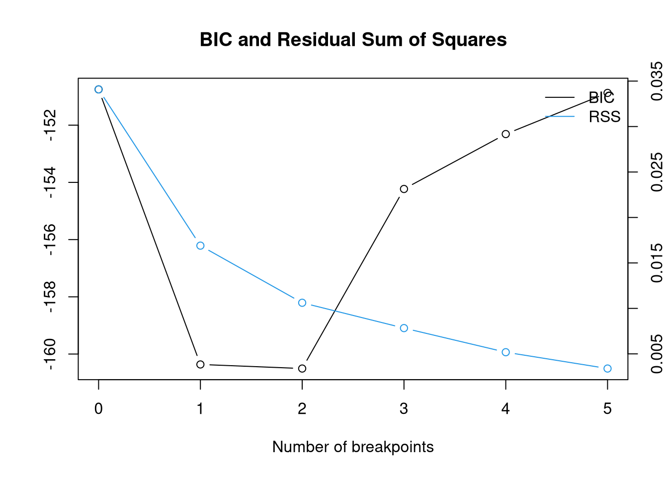
## Phillips curve equation
## estimate breakpoints
bp.pc <- breakpoints(dw ~ dp1 + du + u1, data = uk, h = 5, breaks = 5)
## look at RSS and BIC
plot(bp.pc)

summary(bp.pc)


     Optimal (m+1)-segment partition: 

Call:
breakpoints.formula(formula = dw ~ dp1 + du + u1, h = 5, breaks = 5, 
    data = uk)

Breakpoints at observation number:
                      
m = 1            26   
m = 2         20 28   
m = 3   9        25 30
m = 4   11 16    25 30
m = 5   11 16 22 27 32

Corresponding to breakdates:
                                
m = 1                  1973     
m = 2             1967 1975     
m = 3   1956           1972 1977
m = 4   1958 1963      1972 1977
m = 5   1958 1963 1969 1974 1979

Fit:
                                                                     
m   0          1          2          3          4          5         
RSS  3.409e-02  1.690e-02  1.062e-02  7.835e-03  5.183e-03  3.388e-03
BIC -1.508e+02 -1.604e+02 -1.605e+02 -1.542e+02 -1.523e+02 -1.509e+02

## fit segmented model with three breaks
fac.pc <- breakfactor(bp.pc, breaks = 2, label = "seg")
fm.pc <- lm(dw ~ 0 + fac.pc/dp1 + du + u1, data = uk)
summary(fm.pc)


Call:
lm(formula = dw ~ 0 + fac.pc/dp1 + du + u1, data = uk)

Residuals:
      Min        1Q    Median        3Q       Max 
-0.041392 -0.011516  0.000089  0.010036  0.044539 

Coefficients:
               Estimate Std. Error t value Pr(>|t|)    
fac.pcseg1      0.06574    0.01169   5.623 3.24e-06 ***
fac.pcseg2      0.06231    0.01883   3.310  0.00232 ** 
fac.pcseg3      0.18093    0.05388   3.358  0.00204 ** 
du             -0.14408    0.58218  -0.247  0.80611    
u1             -0.87516    0.37274  -2.348  0.02523 *  
fac.pcseg1:dp1  0.09373    0.24053   0.390  0.69936    
fac.pcseg2:dp1  1.23143    0.20498   6.008 1.06e-06 ***
fac.pcseg3:dp1  0.01618    0.25667   0.063  0.95013    
---
Signif. codes:  0 '***' 0.001 '**' 0.01 '*' 0.05 '.' 0.1 ' ' 1

Residual standard error: 0.02021 on 32 degrees of freedom
Multiple R-squared:  0.9655,    Adjusted R-squared:  0.9569 
F-statistic:   112 on 8 and 32 DF,  p-value: < 2.2e-16

## Results from Table 3 in Bai & Perron (2003):
## coefficient estimates
coef(fm.pc)

    fac.pcseg1     fac.pcseg2     fac.pcseg3             du             u1 
    0.06574278     0.06231337     0.18092502    -0.14408073    -0.87515585 
fac.pcseg1:dp1 fac.pcseg2:dp1 fac.pcseg3:dp1 
    0.09372759     1.23143008     0.01617826

## corresponding standard errors
sqrt(diag(vcov(fm.pc)))

    fac.pcseg1     fac.pcseg2     fac.pcseg3             du             u1 
    0.01169149     0.01882668     0.05388166     0.58217571     0.37273955 
fac.pcseg1:dp1 fac.pcseg2:dp1 fac.pcseg3:dp1 
    0.24052539     0.20497973     0.25666903

## breakpoints and confidence intervals
confint(bp.pc, breaks = 2, het.err = FALSE)


     Confidence intervals for breakpoints
     of optimal 3-segment partition: 

Call:
confint.breakpointsfull(object = bp.pc, breaks = 2, het.err = FALSE)

Breakpoints at observation number:
  2.5 % breakpoints 97.5 %
1    19          20     21
2    27          28     29

Corresponding to breakdates:
  2.5 % breakpoints 97.5 %
1  1966        1967   1968
2  1974        1975   1976