A symbolic description of the model to be fit. This should be of type y ~ x1 + x2 where y should be a matrix with items in the columns and observations in the rows and x1 and x2 are used as partitioning variables. Additionally each item (column) should have the same maximum value (see pctree for a way to handle variable maximum values).
data
a data frame containing the variables in the model.
na.action
a function which indicates what should happen when the data contain missing values (NAs).
deriv
character. If "sum" (the default), the first derivatives of the elementary symmetric functions are calculated with the sum algorithm. Otherwise ("diff") the difference algorithm (faster but numerically unstable) is used.
reltol, maxit
arguments passed via rsmodel to optim.
…
arguments passed to the underlying functions, i.e., to mob_control for rstree, and to the underlying predict and plot methods, respectively.
object, x
an object of class “raschtree”.
newdata
optional data frame with partitioning variables for which predictions should be computed. By default the learning data set is used.
type
character specifying the type of predictions or plot. For the predict method, either just the ID of the terminal “node” can be predicted or some property of the model at a given person parameter (specified by personpar).
personpar
numeric person parameter (of length 1) at which the predictions are evaluated.
terminal_panel, tp_args, tnex, drop_terminal
arguments passed to plot.modelparty/plot.party.
Details
Rating scale trees are an application of model-based recursive partitioning (implemented in mob) to rating scale models (implemented in rsmodel). See Komboz et al. (2018) for a detailed discussion. For technical and algorithmic details, see the documentation of the two core functions linked above as well as vignette(“mob”, package = “partykit”).
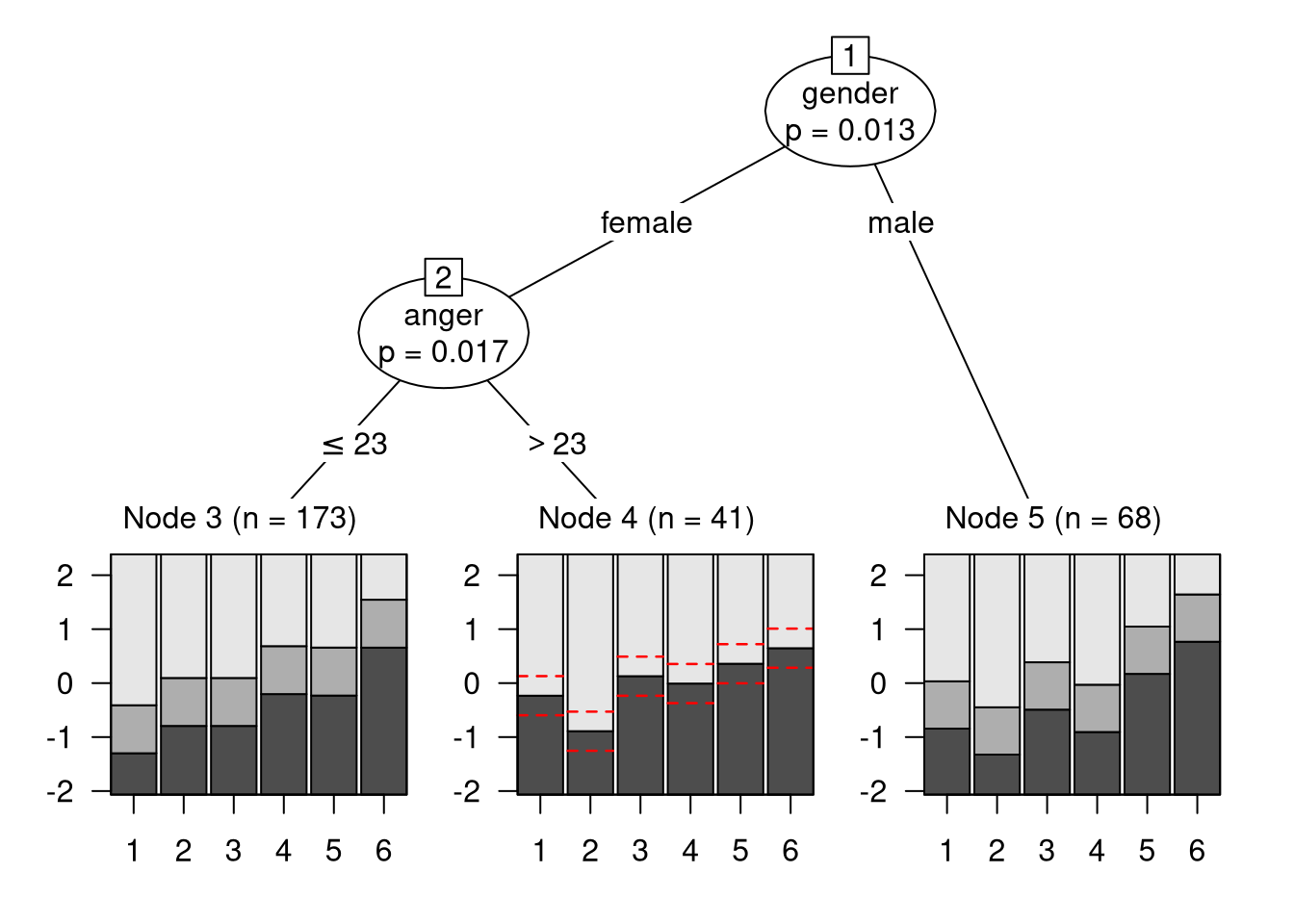
Various methods are provided for “rstree” objects, most of them inherit their behavior from “mob” objects (e.g., print, summary, etc.). For the rating scale models in the nodes of a tree, coef extracts all item parameters. The plot method employs the node_regionplot panel-generating function by default.
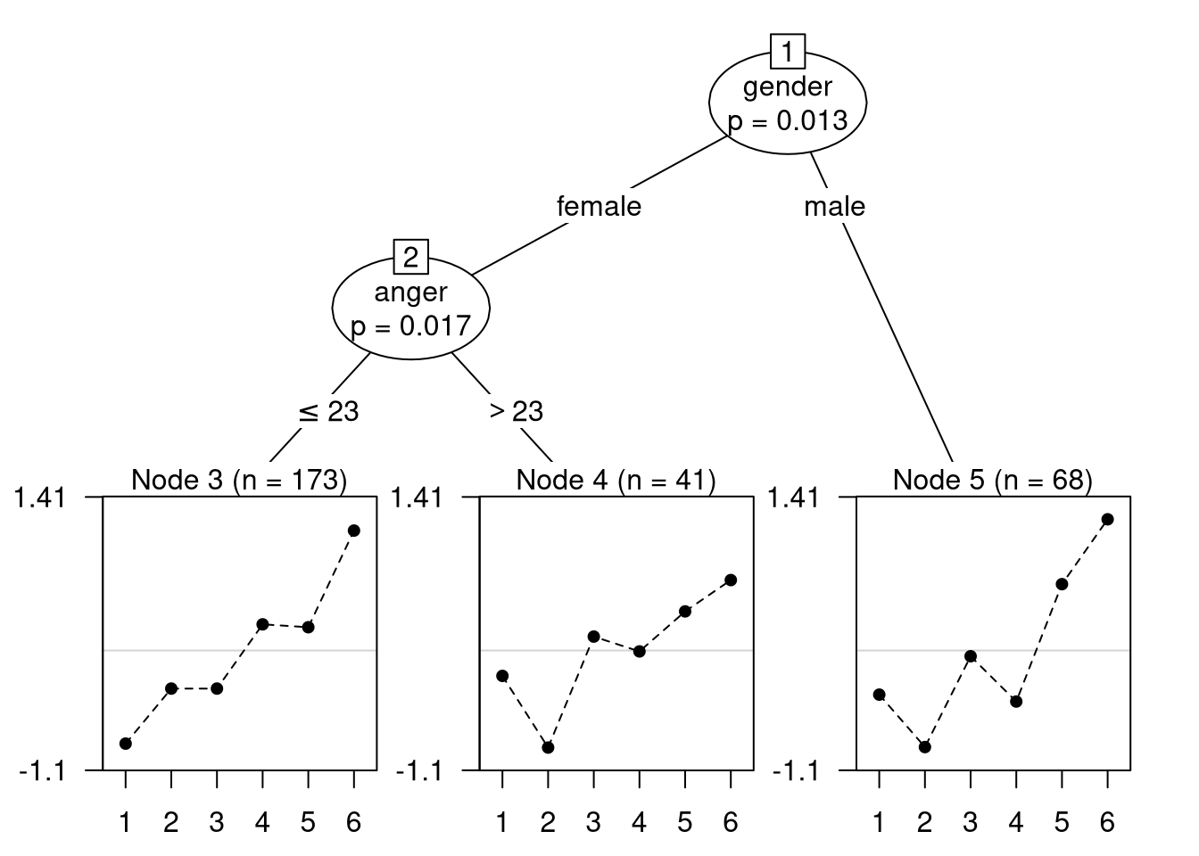
Various methods are provided for “rstree” objects, most of them inherit their behavior from “modelparty” objects (e.g., print, summary, etc.). For the RSMs in the nodes of a tree, coef extracts all item and threshold parameters except those restricted to be zero. itempar and threshpar extract all item and threshold parameters (including the restricted ones). The plot method by default employs the node_regionplot panel-generating function and the node_profileplot panel-generating function is provided as an alternative.
Value
An object of S3 class “rstree” inheriting from class “modelparty”.
References
Komboz B, Zeileis A, Strobl C (2018). Tree-Based Global Model Tests for Polytomous Rasch Models. Educational and Psychological Measurement, 78(1), 128–166. doi:10.1177/0013164416664394
See Also
mob, rsmodel, pctree, raschtree
Examples
library("psychotree")## IGNORE_RDIFF_BEGINo<-options(digits =4)## verbal aggression data from package psychotoolsdata("VerbalAggression", package ="psychotools")## responses to the first other-to-blame situation (bus)VerbalAggression$s1<-VerbalAggression$resp[, 1:6]## exclude subjects who only scored in the highest or the lowest categoriesVerbalAggression<-subset(VerbalAggression, rowSums(s1)>0&rowSums(s1)<12)## fit rating scale tree model for the first other-to-blame situationrst<-rstree(s1~anger+gender, data =VerbalAggression)## print tree (with and without parameters)print(rst)
Rating scale tree

Model formula:
s1 ~ anger + gender

Fitted party:
[1] root
|   [2] gender in female
|   |   [3] anger <= 23: n = 173
|   |         s1S1DoCurse s1S1WantScold   s1S1DoScold s1S1WantShout   s1S1DoShout
|   |              0.5054        0.5054        1.0954        1.0688        1.9563
|   |                  C2
|   |              0.8887
|   |   [4] anger > 23: n = 41
|   |         s1S1DoCurse s1S1WantScold   s1S1DoScold s1S1WantShout   s1S1DoShout
|   |             -0.6582        0.3610        0.2247        0.5922        0.8799
|   |                  C2
|   |             -0.7253
|   [5] gender in male: n = 68
|         s1S1DoCurse s1S1WantScold   s1S1DoScold s1S1WantShout   s1S1DoShout
|            -0.48160       0.35253      -0.06342       1.01438       1.60990
|                  C2
|             0.87640

Number of inner nodes:    2
Number of terminal nodes: 3
Number of parameters per node: 6
Objective function (negative log-likelihood): 975.8
Rating scale tree

Model formula:
s1 ~ anger + gender

Fitted party:
[1] root
|   [2] gender in female
|   |   [3] anger <= 23 *
|   |   [4] anger > 23 *
|   [5] gender in male *

Number of inner nodes:    2
Number of terminal nodes: 3
Number of parameters per node: 6
Objective function (negative log-likelihood): 975.8
## show summary for terminal panel nodessummary(rst)