psychotree

Bradley-Terry Trees

Description

Recursive partitioning (also known as trees) based on Bradley-Terry models.

Usage

bttree(formula, data, na.action, cluster,
  type = "loglin", ref = NULL, undecided = NULL, position = NULL, ...)

## S3 method for class 'bttree'
predict(object, newdata = NULL,
  type = c("worth", "rank", "best", "node"), ...)

Arguments

formula A symbolic description of the model to be fit. This should be of type y ~ x1 + x2 where y should be an object of class paircomp and x1 and x2 are used as partitioning variables.

data an optional data frame containing the variables in the model.

na.action A function which indicates what should happen when the data contain NAs, defaulting to na.pass.

cluster optional vector (typically numeric or factor) with a cluster ID to be employed for clustered covariances in the parameter stability tests.

type character indicating the type of auxiliary model in bttree and the type of predictions in the predict method, respectively. For the auxiliary model see btmodel. For the predict method, four options are available: the fitted “worth” parameter for each alternative, the corresponding “rank”, the “best” alternative or the predicted “node” number.

ref, undecided, position arguments for the Bradley-Terry model passed on to btmodel.

… arguments passed to mob_control.

object fitted model object of class “bttree”.

newdata optionally, a data frame in which to look for variables with which to predict. If omitted, the original observations are used.

Details

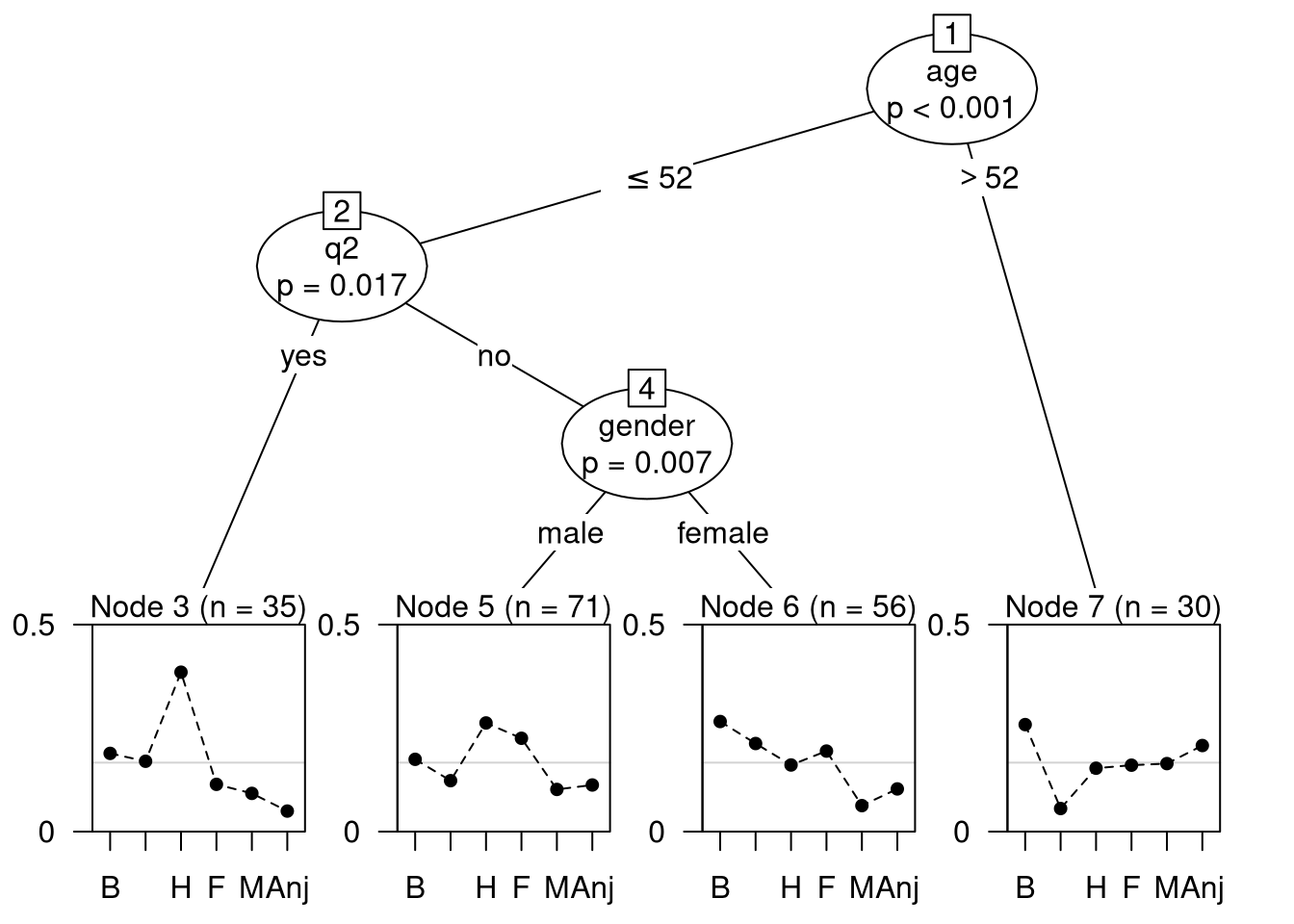
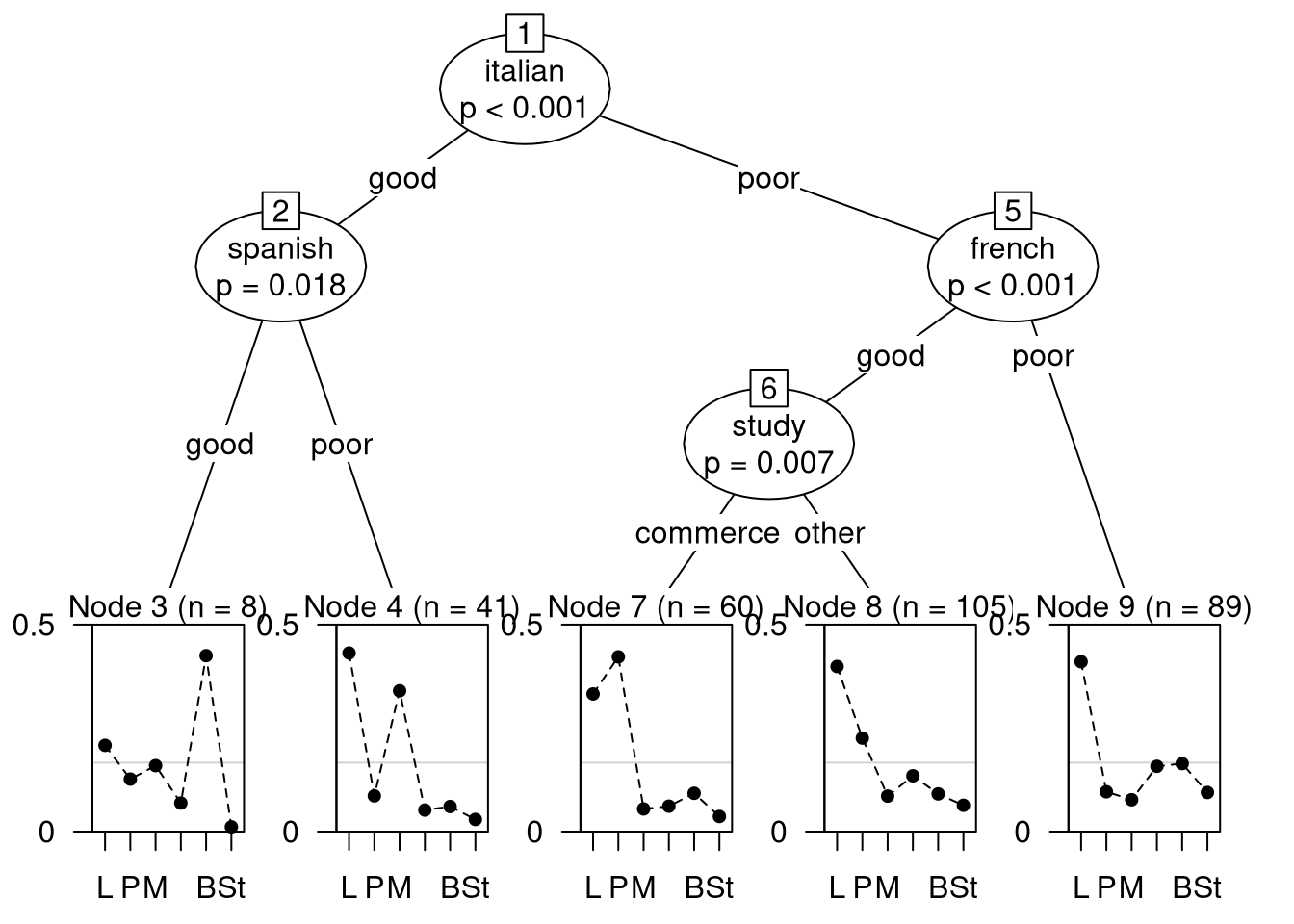
Bradley-Terry trees are an application of model-based recursive partitioning (implemented in mob) to Bradley-Terry models for paired comparison data (implemented in btmodel). Details about the underlying theory and further explanations of the illustrations in the example section can be found in Strobl, Wickelmaier, Zeileis (2011). For technical and algorithmic details, see the documentation of the two core functions linked above as well as vignette(“mob”, package = “partykit”).

Various methods are provided for “bttree” objects, most of them inherit their behavior from “mob” objects (e.g., print, summary, etc.). itempar behaves analogously to coef and extracts the worth/item parameters from the BT models in the nodes of the tree. The plot method employs the node_btplot panel-generating function.

Value

An object of S3 class “bttree” inheriting from class “modelparty”.

References

Strobl C, Wickelmaier F, Zeileis A (2011). Accounting for Individual Differences in Bradley-Terry Models by Means of Recursive Partitioning. Journal of Educational and Behavioral Statistics, 36(2), 135–153. doi:10.3102/1076998609359791

Examples

library("psychotree")

o <- options(digits = 4)

## Germany's Next Topmodel 2007 data
data("Topmodel2007", package = "psychotree")

## BT tree
tm_tree <- bttree(preference ~ ., data = Topmodel2007, minsize = 5, ref = "Barbara")
plot(tm_tree, abbreviate = 1, yscale = c(0, 0.5))

## parameter instability tests in root node
if(require("strucchange")) sctest(tm_tree, node = 1)

            gender       age      q1       q2     q3
statistic 17.08798 3.236e+01 12.6320 19.83922 6.7586
p.value    0.02149 7.915e-04  0.1283  0.00668 0.7452

## worth/item parameters in terminal nodes
itempar(tm_tree)

  Barbara    Anni   Hana  Fiona   Mandy    Anja
3  0.1889 0.16993 0.3851 0.1142 0.09232 0.04958
5  0.1746 0.12305 0.2625 0.2254 0.10188 0.11259
6  0.2659 0.21278 0.1609 0.1945 0.06275 0.10310
7  0.2585 0.05573 0.1531 0.1605 0.16427 0.20792

## CEMS university choice data
data("CEMSChoice", package = "psychotree")
summary(CEMSChoice$preference)

                        >  =   < NA's
London    : Paris     186 26  91    0
London    : Milano    221 26  56    0
Paris     : Milano    121 32  59   91
London    : StGallen  208 22  73    0
Paris     : StGallen  165 19 119    0
Milano    : StGallen  135 28 140    0
London    : Barcelona 217 19  67    0
Paris     : Barcelona 157 37 109    0
Milano    : Barcelona 104 67 132    0
StGallen  : Barcelona 144 25 134    0
London    : Stockholm 250 19  34    0
Paris     : Stockholm 203 30  70    0
Milano    : Stockholm 157 46 100    0
StGallen  : Stockholm 155 50  98    0
Barcelona : Stockholm 172 41  90    0

## BT tree
cems_tree <- bttree(preference ~ french + spanish + italian + study + work + gender + intdegree,
  data = CEMSChoice, minsize = 5, ref = "London")
plot(cems_tree, abbreviate = 1, yscale = c(0, 0.5))

itempar(cems_tree)

  London   Paris  Milano StGallen Barcelona Stockholm
3 0.2083 0.12682 0.15936  0.06905   0.42506   0.01135
4 0.4315 0.08630 0.34017  0.05205   0.06060   0.02939
7 0.3325 0.42215 0.05478  0.06144   0.09252   0.03656
8 0.3989 0.22586 0.08578  0.13480   0.09108   0.06360
9 0.4104 0.09624 0.07697  0.15767   0.16424   0.09451

options(digits = o$digits)