psychotree

Parametric Logisitic (n-PL) IRT Model Trees

Description

Recursive partitioning (also known as trees) based on parametric logistic (n-PL) item response theory (IRT) models for global testing of differential item functioning (DIF).

Usage

npltree(formula, data, type = c("Rasch", "1PL", "2PL", "3PL", "3PLu", "4PL"),
  start = NULL, weights = NULL, grouppars = FALSE,
  vcov = TRUE, method = "BFGS", maxit = 500L,
  reltol = 1e-10, deriv = "sum", hessian = TRUE,
  full = TRUE, minsize = NULL, ...)

## S3 method for class 'npltree'
plot(x, type = c("profile", "regions"), terminal_panel = NULL,
  tp_args = list(...), tnex = 2L, drop_terminal = TRUE, ...)

Arguments

formula A symbolic description of the model to be fit. This should be of type y ~ x1 + x2 where y should be an item response matrix and x1 and x2 are used as partitioning variables. For the models estimated using marginal maximum likelihood (MML), it is additionally poosible to allow for impact of a group variable so that different ability distributions are estimated in each group. This can be specified by extending the previous formula by a group factor g as y ~ g | x1 + x2.

data a data frame containing the variables in the model.

type character, specifying either the type of IRT model in npltree (see also nplmodel) or the type of visualization to be used in the plot method, respectively.

start an optional vector or list of starting values (see raschmodel or nplmodel).

weights an optional vector of weights (interpreted as case weights).

grouppars logical. Should the estimated distributional group parameters of a multiple-group model be included in the model parameters? (See nplmodel.)

vcov logical or character specifying the type of variance-covariance matrix (if any) computed for the final models when fitted using MML (see nplmodel).

method control parameter for the optimizer used by mirt for the EM algorithm when models are fitted using MML (see nplmodel).

maxit control parameter for the optimizer used by raschmodel or nplmodel (see raschmodel, nplmodel).

reltol control parameter for the optimizer used by raschmodel or nplmodel (see raschmodel, nplmodel).

deriv character. Which type of derivatives should be used for computing gradient and Hessian matrix when fitting Rasch models with the conditional maximum likelihood (CML) method (see raschmodel)?

hessian logical. Should the Hessian be computed for Rasch models fitted with the CML method (see raschmodel)?

full logical. Should a full model object be returned for Rasch models fitted with the CML method (see raschmodel)?

minsize The minimum number of observations in each node, which is passed to mob_control. If not set, it is 300 for 2PL models and 500 for 3PL, 3PLu, and 4PL models.

… arguments passed to mob_control for npltree, and to the underlying plot method.

x an object of class npltree.

terminal_panel, tp_args, tnex, drop_terminal arguments passed to mob.

Details

Parametric logistic (n-PL) model trees are an application of model-based recursive partitioning (implemented in mob) to item response theory (IRT) models (implemented in raschmodel and nplmodel). While the “Rasch” model is estimated by conditional maximum likelihood (CML) all other n-PL models are estimated by marginal maximum likelihood (MML) via the standard EM algorithm. The latter allow the specification of multiple-group model to capture group impact on the ability distributions.

For technical and algorithmic details, see the documentation of the core functions linked above as well as vignette(“mob”, package = “partykit”).

Various methods are provided for “npltree” objects, most of them inherit their behavior from “modelparty” objects (e.g., print, summary). Additionally, dedicated extractor functions or provided for the different groups of model parameters in each node of the tree: itempar (item parameters), threshpar (threshold parameters), guesspar (guessing parameters), upperpar (upper asymptote parameters).

Value

An object of S3 class “npltree” inheriting from class “modelparty”.

Examples

library("psychotree")

o <- options(digits = 4)

# fit a Rasch (1PL) tree on the SPISA data set
library("psychotree")
data("SPISA", package = "psychotree")
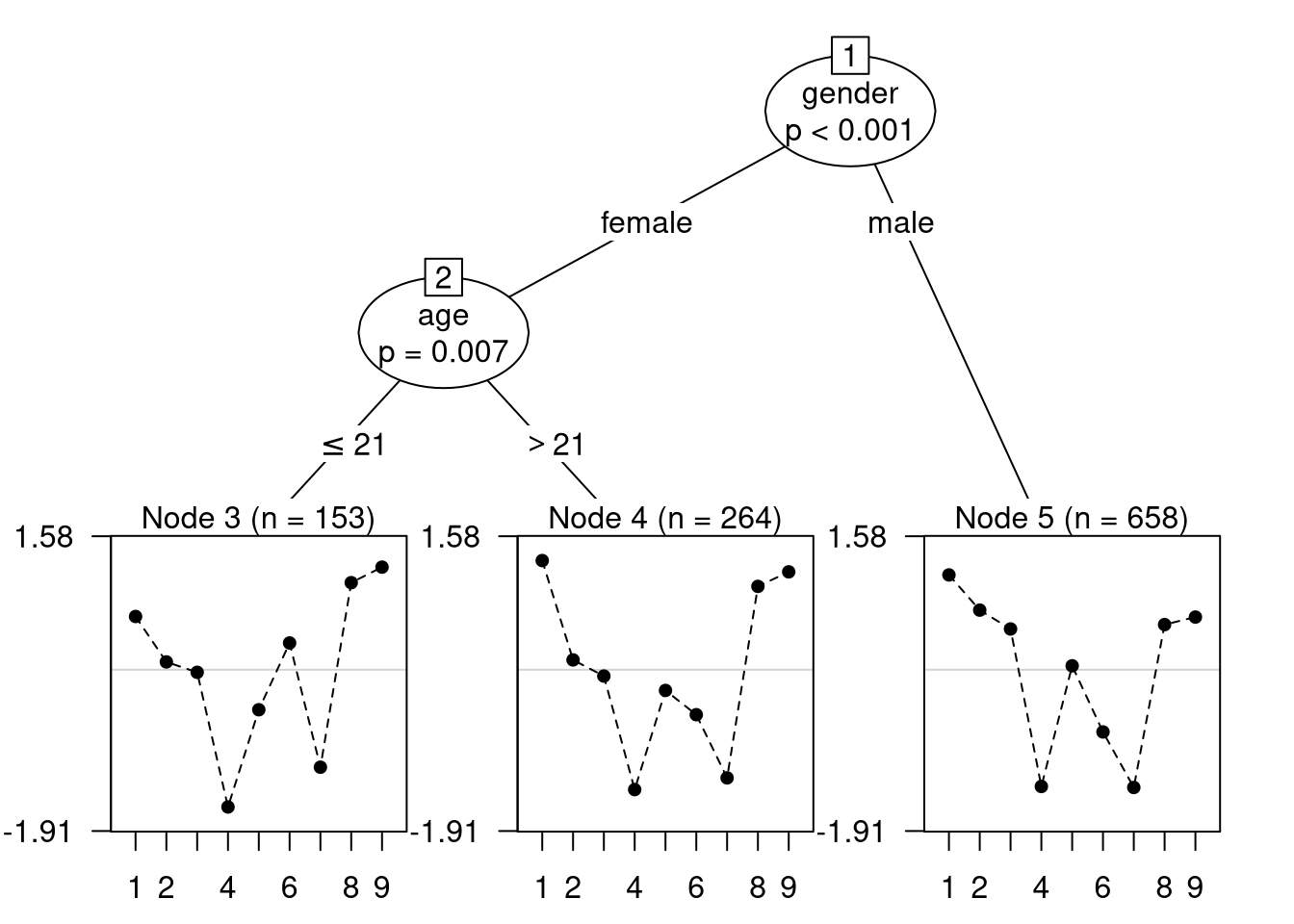
nplt <- npltree(spisa[, 1:9] ~ age + gender + semester + elite + spon, 
  data = SPISA, type = "Rasch")
nplt

PL Tree

Model formula:
spisa[, 1:9] ~ age + gender + semester + elite + spon

Fitted party:
[1] root
|   [2] gender in female
|   |   [3] age <= 21: n = 153
|   |       `spisa[, 1:9]`2 `spisa[, 1:9]`3 `spisa[, 1:9]`4 `spisa[, 1:9]`5 `spisa[, 1:9]`6 
|   |               -0.5380         -0.6611         -2.2553         -1.1041         -0.3135 
|   |       `spisa[, 1:9]`7 `spisa[, 1:9]`8 `spisa[, 1:9]`9 
|   |               -1.7846          0.4007          0.5844 
|   |   [4] age > 21: n = 264
|   |       `spisa[, 1:9]`2 `spisa[, 1:9]`3 `spisa[, 1:9]`4 `spisa[, 1:9]`5 `spisa[, 1:9]`6 
|   |               -1.1765         -1.3674         -2.7117         -1.5377         -1.8251 
|   |       `spisa[, 1:9]`7 `spisa[, 1:9]`8 `spisa[, 1:9]`9 
|   |               -2.5733         -0.3057         -0.1337 
|   [5] gender in male: n = 658
|       `spisa[, 1:9]`2 `spisa[, 1:9]`3 `spisa[, 1:9]`4 `spisa[, 1:9]`5 `spisa[, 1:9]`6 
|               -0.4169         -0.6400         -2.5050         -1.0763         -1.8594 
|       `spisa[, 1:9]`7 `spisa[, 1:9]`8 `spisa[, 1:9]`9 
|               -2.5169         -0.5883         -0.4991 

Number of inner nodes:    2
Number of terminal nodes: 3
Number of parameters per node: 8
Objective function (negative log-likelihood): 3529

# visualize
plot(nplt)

# compute summaries of the models fitted in nodes 1 and 2
summary(nplt, 1:2)

$`1`

Rasch model

Difficulty parameters:
                Estimate Std. Error z value Pr(>|z|)    
`spisa[, 1:9]`2  -0.6159     0.0997   -6.18  6.6e-10 ***
`spisa[, 1:9]`3  -0.8202     0.0994   -8.25  < 2e-16 ***
`spisa[, 1:9]`4  -2.5164     0.1099  -22.90  < 2e-16 ***
`spisa[, 1:9]`5  -1.1947     0.0996  -12.00  < 2e-16 ***
`spisa[, 1:9]`6  -1.5974     0.1010  -15.82  < 2e-16 ***
`spisa[, 1:9]`7  -2.3956     0.1082  -22.15  < 2e-16 ***
`spisa[, 1:9]`8  -0.3958     0.1005   -3.94  8.2e-05 ***
`spisa[, 1:9]`9  -0.2846     0.1010   -2.82   0.0048 ** 
---
Signif. codes:  0 '***' 0.001 '**' 0.01 '*' 0.05 '.' 0.1 ' ' 1

Log-likelihood: -3580 (df = 8) 
Number of iterations in BFGS optimization: 13 


$`2`

Rasch model

Difficulty parameters:
                Estimate Std. Error z value Pr(>|z|)    
`spisa[, 1:9]`2  -0.9247     0.1641   -5.63  1.8e-08 ***
`spisa[, 1:9]`3  -1.0909     0.1634   -6.67  2.5e-11 ***
`spisa[, 1:9]`4  -2.5234     0.1725  -14.63  < 2e-16 ***
`spisa[, 1:9]`5  -1.3606     0.1631   -8.34  < 2e-16 ***
`spisa[, 1:9]`6  -1.2642     0.1631   -7.75  9.1e-15 ***
`spisa[, 1:9]`7  -2.2626     0.1687  -13.42  < 2e-16 ***
`spisa[, 1:9]`8  -0.0309     0.1757   -0.18     0.86    
`spisa[, 1:9]`9   0.1452     0.1798    0.81     0.42    
---
Signif. codes:  0 '***' 0.001 '**' 0.01 '*' 0.05 '.' 0.1 ' ' 1

Log-likelihood: -1420 (df = 8) 
Number of iterations in BFGS optimization: 13

options(digits = o$digits)