A symbolic description of the model to be fit. This should be of type y ~ x1 + x2 where y should be a binary 0/1 item response matrix and x1 and x2 are used as partitioning variables.
data
a data frame containing the variables in the model.
na.action
a function which indicates what should happen when the data contain missing values (NAs).
deriv
character. Which type of derivatives should be used for computing gradient and Hessian matrix? Analytical with sum algorithm (“sum”), analytical with difference algorithm (“diff”, faster but numerically unstable), or numerical. Passed to raschmodel.
reltol, maxit
arguments passed via raschmodel to optim.
…
arguments passed to the underlying functions, i.e., to mob_control for raschtree, and to the underlying predict and plot methods, respectively.
object, x
an object of class “raschtree”.
newdata
optional data frame with partitioning variables for which predictions should be computed. By default the learning data set is used.
type
character specifying the type of predictions or plot. For the predict method, either just the ID of the terminal “node” can be predicted or some property of the model at a given person parameter (specified by personpar).
personpar
numeric person parameter (of length 1) at which the predictions are evaluated.
terminal_panel, tp_args, tnex, drop_terminal
arguments passed to plot.modelparty/plot.party.
Details
Rasch trees are an application of model-based recursive partitioning (implemented in mob) to Rasch models (implemented in raschmodel). See Strobl et al. (2015) for a detailed discussion. For technical and algorithmic details, see the documentation of the two core functions linked above as well as vignette(“mob”, package = “partykit”).
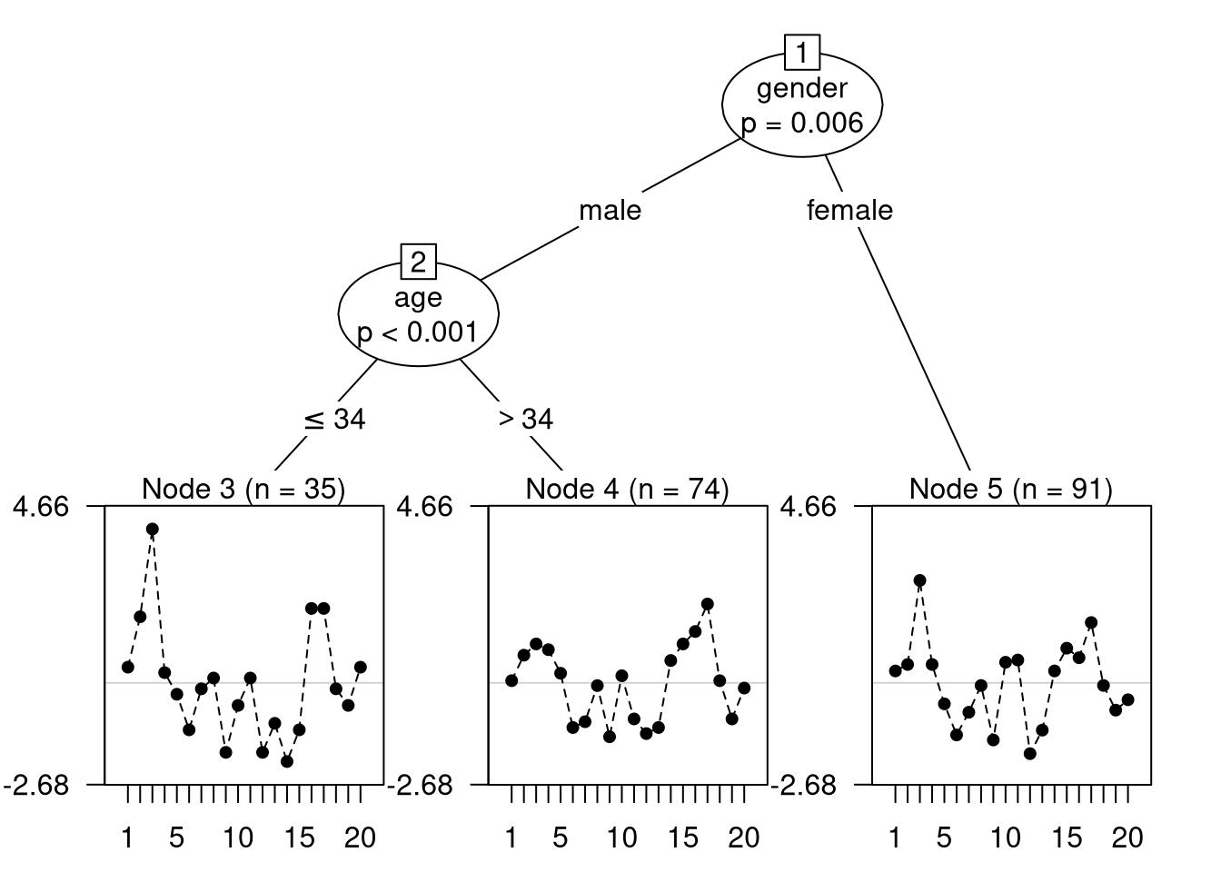
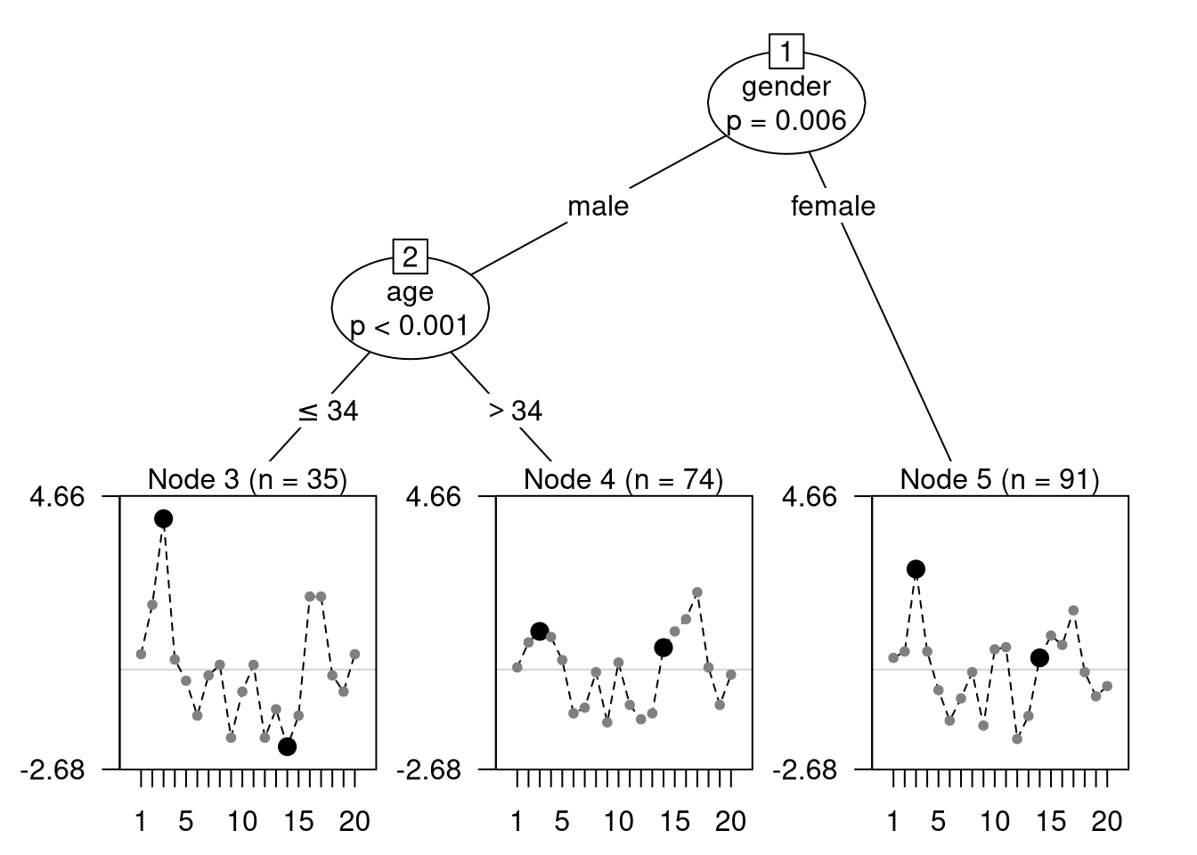
Various methods are provided for “raschtree” objects, most of them inherit their behavior from “modelparty” objects (e.g., print, summary, etc.). For the Rasch models in the nodes of a tree, coef extracts all item parameters except the first one which is always restricted to be zero. itempar extracts all item parameters (including the first one) and by default restricts their sum to be zero (but other restrictions can be used as well). The plot method by default employs the node_profileplot panel-generating function and the node_regionplot panel-generating function is provided as an alternative.
Rasch tree models are introduced in Strobl et al. (2015), whose analysis for the SPISA data is replicated in vignette(“raschtree”, package = “psychotree”). Their illustration employing artificial data is replicated below.
Value
An object of S3 class “raschtree” inheriting from class “modelparty”.
References
Strobl C, Kopf J, Zeileis A (2015). Rasch Trees: A New Method for Detecting Differential Item Functioning in the Rasch Model. Psychometrika, 80(2), 289–316. doi:10.1007/s11336-013-9388-3
See Also
mob, raschmodel, rstree, pctree
Examples
library("psychotree")o<-options(digits =4)## artificial datadata("DIFSim", package ="psychotree")## fit Rasch tree modelrt<-raschtree(resp~age+gender+motivation, data =DIFSim)plot(rt)