install.packages("psychotree")Using the raschtree Function for Detecting Differential Item Functioning in the Rasch Model
Abstract
The psychotree package contains the function raschtree, that can be used to detect differential item functioning (DIF) in the Rasch model. The DIF detection method implemented in raschtree is based on the model-based recursive partitioning framework of Zeileis et al. (2008) and employs generalized M-fluctuation tests (Zeileis and Hornik 2007) for detecting differences in the item parameters between different groups of subjects. The statistical methodology behind raschtree is described in detail in Strobl et al. (2015). The main advantage of this approach is that it allows to detect groups of subjects exhibiting DIF, that are not pre-specified, but are detected automatically from combinations of covariates. In this vignette, the practical usage of raschtree is illustrated.
Differential item functioning in the Rasch model
A key assumption of the Rasch model is that the item parameter estimates should not depend on the person sample (and vice versa). This assumption may be violated if certain items are easier or harder to solve for certain groups of subjects - regardless of their true ability - in which case we speak of differential item functioning (DIF).
In order to detect DIF with the raschtree function, the item responses and all covariates that should be tested for DIF need to be handed over to the method, as described below. Then the following steps are conducted:
- At first, one joint Rasch model is fit for all subjects.
- Then it is tested statistically whether the item parameters differ along any of the covariates.
- In that case the sample is split along that covariate and two separate Rasch model s are estimated.
- This process is repeated as long as there is further DIF (and the subsample is still large enough).
For details on the underlying statistical framework implemented in raschtree see Strobl et al. (2015).
The main advantage of the Rasch tree approach is that DIF can be detected between groups of subjects created by more than one covariate. For example, certain items may be easier for male subjects over the age of 40 as opposed to all other subjects. In this case DIF is associated with an interaction of the variables gender and age, rather than any one variable alone.
Moreover, with this approach it is not necessary to pre-define cutpoints in continuous variables, as would be the standard approach when using, e.g., a likelihood ratio or Wald test: Usually, age groups are pre-specified, for example by means of splitting at the median. However, the median may not be where the actual parameter change occurs - it could be that only very young or very old subjects find certain items particularly easy or hard. By splitting at the median this effect may be disguised. Therefore, the Rasch tree method searches for the value corresponding to the strongest parameter change and splits the sample at that value. Certain statistical techniques are necessary for doing this in a statistically sound way, as described in detail in Strobl et al. (2015).
Now the practical application of raschtree is outlined, starting with the data preparation.
Data preparation
When using raschtree for the first time, the psychotree package needs to be installed first:
After this, the package is permanently installed on the computer, but needs to be made available at the start of every new R session:
library("psychotree")The package contains a data example for illustrating the Rasch trees, that can be loaded with:
data("SPISA", package = "psychotree")The data set SPISA consists of the item responses and covariate values of 1075 subjects. It is a subsample of a larger data set from an online quiz, that was carried out by the German weekly news magazine SPIEGEL in 2009 via the online version of the magazine SPIEGEL Online (SPON). The quiz was designed for testing one’s general knowledge and consisted of a total of 45 items from five different topics: politics, history, economy, culture and natural sciences. A thorough analysis and discussion of the original data set is provided in Trepte and Verbeet (2010).
The data are structured in the following way: The variable spisa contains the 0/1-responses of all subjects to all test items (i.e., spisa is only a single variable but contains a matrix of responses). In addition to that, covariates like age and gender are available for each subject:
Item reponsesspisa
|
Covariatesgender
|
age
|
semester
|
elite
|
spon
|
||||||||||
|---|---|---|---|---|---|---|---|---|---|---|---|---|---|---|---|
| 1 | 0 | 0 | 1 | 1 | \(\cdots\) | 0 | 1 | 1 | 1 | 1 | female | 21 | 3 | no | 1-3/month |
| 0 | 1 | 0 | 1 | 1 | \(\cdots\) | 1 | 1 | 1 | 1 | 1 | male | 20 | 1 | no | 4-5/week |
| 0 | 0 | 0 | 1 | 0 | \(\cdots\) | 0 | 1 | 1 | 1 | 1 | female | 25 | 9 | no | 1-3/month |
| 0 | 0 | 1 | 1 | 1 | \(\cdots\) | 1 | 1 | 0 | 1 | 1 | male | 27 | 10 | no | never |
| 1 | 1 | 1 | 1 | 1 | \(\cdots\) | 0 | 0 | 1 | 1 | 1 | male | 24 | 8 | no | 1/week |
| 1 | 0 | 0 | 1 | 0 | \(\cdots\) | 1 | 1 | 0 | 1 | 1 | male | 20 | 1 | yes | 1-3/month |
| \(\vdots\) | \(\vdots\) | \(\vdots\) | \(\vdots\) | \(\vdots\) | \(\vdots\) |
If your own data set, termed for example mydata, is in a different format, it is easy to change it into the right format for raschtree. For example, if the item responses are coded as individual variables like this:
Item reponsesitem1
|
item2
|
item3
|
item4
|
item5
|
Covariatesgender
|
age
|
semester
|
|---|---|---|---|---|---|---|---|
| 1 | 0 | 0 | 1 | 1 | female | 21 | 3 |
| 0 | 1 | 0 | 1 | 1 | male | 20 | 1 |
| 0 | 0 | 0 | 1 | 0 | female | 25 | 9 |
| 0 | 0 | 1 | 1 | 1 | male | 27 | 10 |
| 1 | 1 | 1 | 1 | 1 | male | 24 | 8 |
You can bring them into a more convenient format by first defining a new variable resp that contains the matrix of item responses (i.e., the first five columns of mydata):
mydata$resp <- as.matrix(mydata[ , 1:5])Then you can omit the original separate item response variables from the data set
mydata <- mydata[ , -(1:5)]The data set then contains both the complete matrix of item responses - termed resp - and the covariates as individual columns, so that later it is easier to address the complete matrix of item responses in the function call.
Now the data preparation is done and we can fit a Rasch tree.
Model fitting, plotting and extraction of parameter values
The idea of Rasch trees is to model differences in the Rasch model for the item responses by means of the covariates. This idea translates intuitively into the formula interface that is commonly used in R functions, such as lm for linear models: In a linear model, where the response variable y is modeled by the covariates x1 and x2, the formula in R looks like this:
y ~ x1 + x2
Very similarly, in the Rasch tree for our SPISA data, where the item responses spisa are modeled by the covariates age, gender, semester, elite and spon, the formula used in raschtree looks like this:
spisa ~ age + gender + semester + elite + spon
The complete call is
my_first_raschtree <- raschtree(spisa ~ age + gender +
  semester + elite + spon, data = SPISA)
Note that the model is not only fitted, but also saved under the name my_first_raschtree, so that we can later extract information from the fitted model object and plot the Rasch tree.
As a shortcut, when all other variables in the data set are to be used as covariates, as in our example, the covariates do not have to be listed explicitly in the formula but can replaced by a dot, as in raschtree(spisa ~ ., data = SPISA) (leading to equivalent output as the call above). Moreover, if you want to see the process of the Rasch tree fitting, including the computation of the \(p\)-values and corresponding split decisions in each step, you can use the verbose option, as in raschtree(spisa ~ ., data = SPISA, verbose = TRUE). The verbose option also has the advantage that you can see something happening on your screen when raschtree takes a while to complete - which may be the case if there are many variables with DIF and if these variables offer many possible cutpoints, like continuous variables and factors with many categories.
In case you receive an error message, one possible cause is that certain nodes in the Rasch tree contain too few observations to actually fit a Rasch model. In this case it might be necessary to restrict the minimum number of observations per node to a higher value by means of the minsize argument:
my_first_raschtree <- raschtree(spisa ~ age + gender +
  semester + elite + spon, data = SPISA, minsize = 30)
Note that while the minimum number of observations per node, minsize, should be chosen large enough to fit the model, it should not be chosen unnecessarily large, because otherwise splits at the margins of the feature space cannot be selected.
The resulting Rasch tree can then be plotted with the generic plot call:
plot(my_first_raschtree)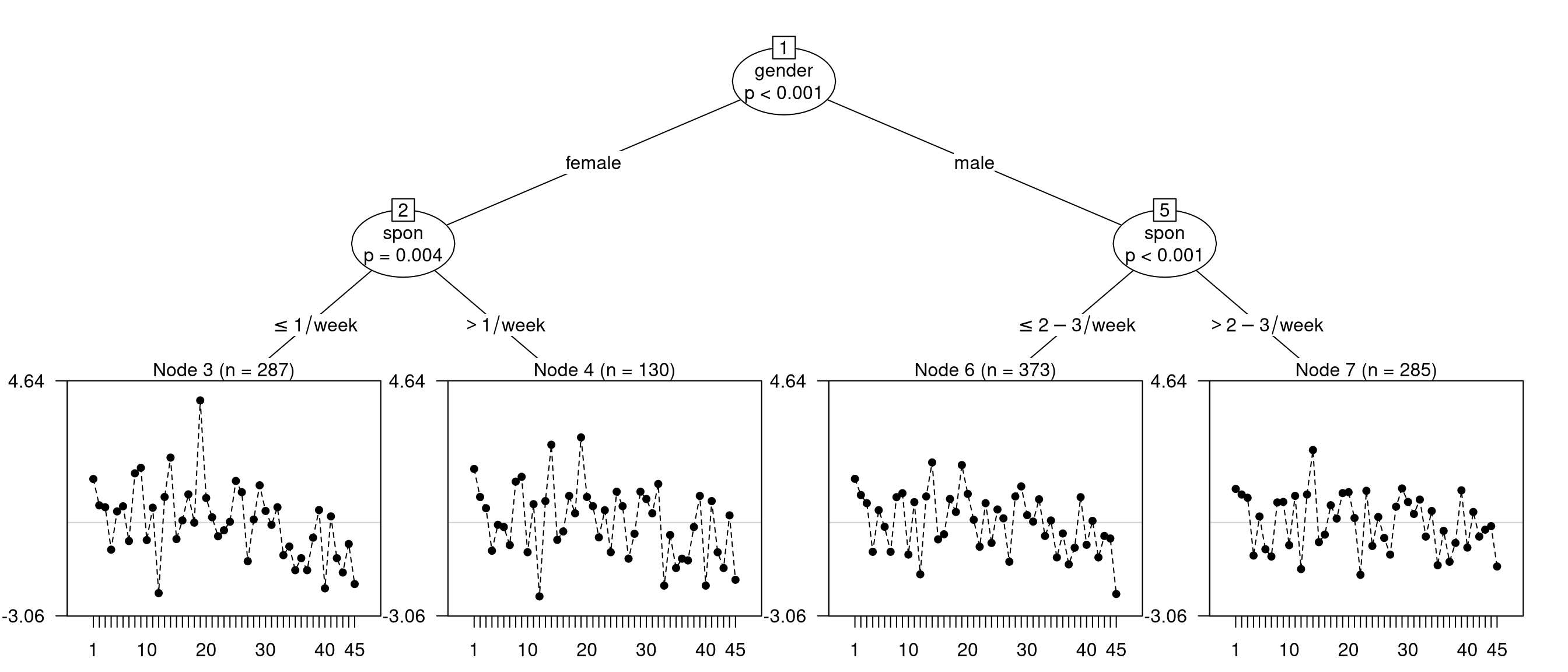
The plot function also accepts many options for standard plot functions, including coloring. Here, a qualitative color palette is employed to indicate the blocks of nine items from each of the five different topics covered in the quiz: politics, history, economy, culture and natural sciences:
plot(my_first_raschtree,
      col = rep(palette.colors(5), each = 9))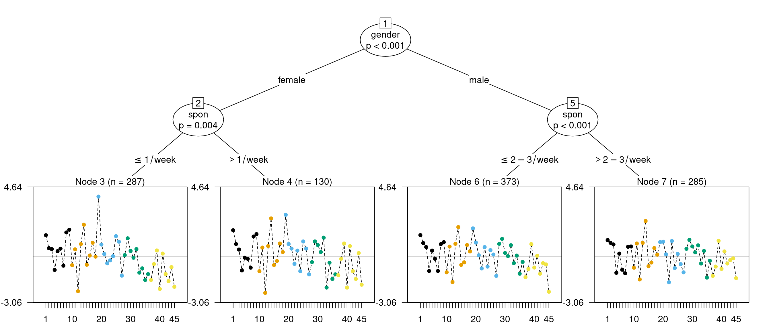
For extracting the estimated item parameters for each group, there are two different calls corresponding to the two different ways to scale the item parameters: The parameters of a Rasch model are unique only up to linear transformations. In particular, the origin of the scale is not fixed but chosen arbitrarily. There are two common ways to choose the origin: setting one item parameter to zero or setting the sum of all item parameters to zero. Accordingly, there are two calls to extract the item parameters from raschtree one way or the other:
coef(my_first_raschtree, node = 4)
##     spisa2     spisa3     spisa4     spisa5     spisa6     spisa7     spisa8
## -0.9187137 -1.2874521 -2.6805353 -1.8312493 -1.9026320 -2.4951461 -0.4162699
##     spisa9    spisa10    spisa11    spisa12    spisa13    spisa14    spisa15
## -0.2581010 -2.7296693 -1.1543021 -4.1769262 -1.0539421  0.7916895 -2.3241647
##    spisa16    spisa17    spisa18    spisa19    spisa20    spisa21    spisa22
## -2.0495272 -0.8845425 -1.4541652  1.0321505 -0.9187137 -1.2208998 -2.2428880
##    spisa23    spisa24    spisa25    spisa26    spisa27    spisa28    spisa29
## -1.3540086 -2.7296693 -0.7458437 -1.2208998 -2.9403761 -2.1253688 -0.7458437
##    spisa30    spisa31    spisa32    spisa33    spisa34    spisa35    spisa36
## -0.9865644 -1.4541652 -0.4922363 -3.8232693 -2.1640318 -3.2469996 -2.9403761
##    spisa37    spisa38    spisa39    spisa40    spisa41    spisa42    spisa43
## -2.9972355 -1.9026320 -0.8845425 -3.8232693 -1.0539421 -2.7296693 -3.2469996
##    spisa44    spisa45
## -1.5213581 -3.6324888
where the parameter for the first item is set to zero and therefore not displayed (the call is termed coef, because that is the name of the call extracting the estimated parameters, or coefficients, from standard regression models generated, e.g., with the lm function) and
itempar(my_first_raschtree, node = 4)
##      spisa1      spisa2      spisa3      spisa4      spisa5      spisa6
##  1.75417311  0.83545944  0.46672105 -0.92636220 -0.07707618 -0.14845889
##      spisa7      spisa8      spisa9     spisa10     spisa11     spisa12
## -0.74097296  1.33790319  1.49607208 -0.97549614  0.59987100 -2.42275309
##     spisa13     spisa14     spisa15     spisa16     spisa17     spisa18
##  0.70023103  2.54586259 -0.56999156 -0.29535409  0.86963065  0.30000788
##     spisa19     spisa20     spisa21     spisa22     spisa23     spisa24
##  2.78632359  0.83545944  0.53327329 -0.48871486  0.40016448 -0.97549614
##     spisa25     spisa26     spisa27     spisa28     spisa29     spisa30
##  1.00832941  0.53327329 -1.18620295 -0.37119569  1.00832941  0.76760868
##     spisa31     spisa32     spisa33     spisa34     spisa35     spisa36
##  0.30000788  1.26193682 -2.06909621 -0.40985866 -1.49282653 -1.18620295
##     spisa37     spisa38     spisa39     spisa40     spisa41     spisa42
## -1.24306243 -0.14845889  0.86963065 -2.06909621  0.70023103 -0.97549614
##     spisa43     spisa44     spisa45
## -1.49282653  0.23281497 -1.87831571
where the item parameters by default sum to zero (other restrictions can be specified as well).
Here the item parameters have been displayed only for the subjects in node number 4 (representing female students who access the online magazine more than once per week) to save space. The item parameters for all groups can be displayed by omitting the node argument.
Interpretation
Ideally, if none of the items showed DIF, we would find a tree with only one single node. In this case, one joint Rasch model would be appropriate to describe the entire data set. (But note that - like all statistical methods based on significance tests - Rasch trees have power to detect DIF only if the sample size is large enough.)
If, however, the Rasch tree shows at least one split, this indicates that DIF is present and that it is not appropriate to compare the different groups of subjects with the test without accounting for it. DIF may be caused by certain characteristics of the items, such as their wording. In practice, items showing DIF are often excluded from the test. Sometimes it may also be possible to rephrase the items to resolve the DIF.
If several items show the same DIF pattern, this may also indicate that they measure a secondary dimension in addition to the primary dimension. An example could be word problems in a math test, that also measure reading ability. If multiple dimensions are of interest, a multidimensional model can be used, see packages mirt and TAM Robitzsch et al. (2020). Note, however, that whether multidimensionality can be detected always depends not only on the items, but also on whether the persons in the sample used for validating the test actually show variation on the different dimensions.
Finally note that when one joint, unidimensional Rasch model is not appropriate to describe the entire test, this also means that a ranking of the subjects based on the raw scores (i.e., the number of items that each subject answered correctly) is not appropriate either, because this would also assume that the test is unidimensional.
Stability assessment
A tree based on a single sample does not provide any assessment of the confidence we should have in its interpretation - e.g., as we would be used to in parametric models by inspecting the confidence intervals for parameter estimates. However, a toolkit for assessing the stability of trees based on resampling is now provided by the stablelearner package (Philipp et al. 2016).
Starting from version 0.1-2, stablelearner offers descriptive and graphical analyses of the variable and cutpoint selection of trees for psychometric models, including Rasch trees, fitted via the psychotree package (note that this requires at least version 0.6-0 of the psychotools package, which is used internally for fitting the models).
This descriptive and graphical analysis of the variable and cutpoint selection can be performed by using the stabletree function, which repeatedly draws random samples from the training data, refits the tree, and displays a summary of the variable and cutpoint selection over the samples. This can give us an intuition of how similar or dissimilar the results would have been for different random samples.
The package has to be installed (once), e.g., via
install.packages("stablelearner")and then activated (each time) for the current session using
library("stablelearner")Then, we can easily assess the stability of the Rasch tree my_first_raschtree by using the stabletree function.
We set a seed for the random number generator to make the analysis based on random draws from the training data reproducible. By default, stabletree performs subsampling with a fraction of v = 0.632 of the original training data and refits 500 trees. Here, we only refit B = 50 trees to save time, but still this computation can take a while.
set.seed(4321)
my_first_raschtree_st <- stabletree(my_first_raschtree, B = 50)
In case you receive an error message, again this may be due to a too small sample size for fitting the model in certain nodes. Even if in the original tree all nodes were big enough to estimate the model, due to the random sampling in stabletree, smaller nodes can result in some random samples. In order to prevent this, the minimum node size minsize needs to be increased already in the raschtree command, before applying stabletree, because the settings of the original Rasch tree are passed on to stabletree.
The function stabletree returns an object of class stabletree, for which a summary method and several plot methods exist:
summary(my_first_raschtree_st)
##
## Call:
## raschtree(formula = spisa ~ age + gender + semester + elite +
##     spon, data = SPISA, minsize = 30)
##
## Sampler:
## B = 50
## Method = Subsampling with 63.2% data
##
## Variable selection overview:
##
##          freq * mean *
## gender   1.00 1 1.00 1
## spon     0.60 1 0.82 2
## semester 0.18 0 0.18 0
## age      0.04 0 0.04 0
## elite    0.02 0 0.02 0
## (* = original tree)
The summary prints the relative variable selection frequencies (freq) as well as the average number of splits in each variable (mean) over all 50 trees. A relative variable selection frequency of one means that a variable was selected in each of the 50 trees. The average number of splits can show values greater than 1 if the same variable is used more than once in the same tree. The asterisk columns indicate whether this variable was selected in the original tree, and how often. For example, the variable gender was selected as a splitting variable once in every tree, including the original tree. The variable spon, on the other had, was selected in 60% of the trees, also in the orignal tree, on average 0.82 times, but twice in the original tree.
By using barplot, we can also visualize the variable selection frequencies:
barplot(my_first_raschtree_st)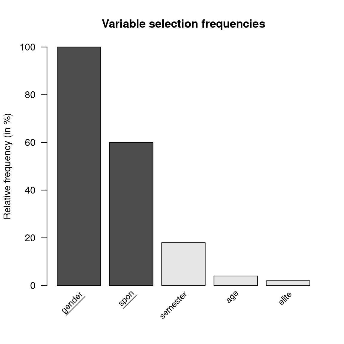
Here the variables that were included in the original tree are marked by darker shading and underlined variable names. We see again that most trees agreed on the two most relevant splitting variables, gender and spon.
The additional function image allows for a more detailed visualization of the variable selection patterns, that are displayed as one row on the y-axis for each of the 50 trees:
image(my_first_raschtree_st)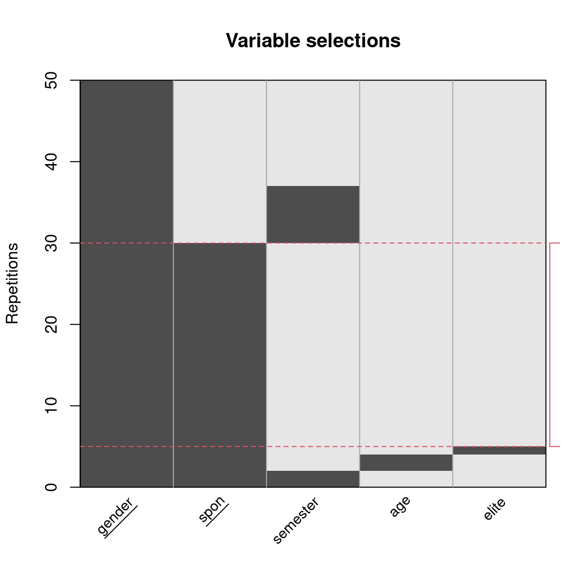
We observe again that about half of the 50 trees have selected the same combination of variables, gender and spon, that was also selected in the original tree. This combination of variables selected by the original tree is framed in red. Other combinations that were selected by larger groups of trees were, e.g., gender alone, gender and semester, gender, spon and age as well as gender, spon and semester.
Finally, the plot function allows us to inspect the cutpoints and resulting partitions for each variable over all 50 trees, with the variables included in the original tree again marked by underlined variable names and the cutpoints from the original trees indicated in red:
plot(my_first_raschtree_st)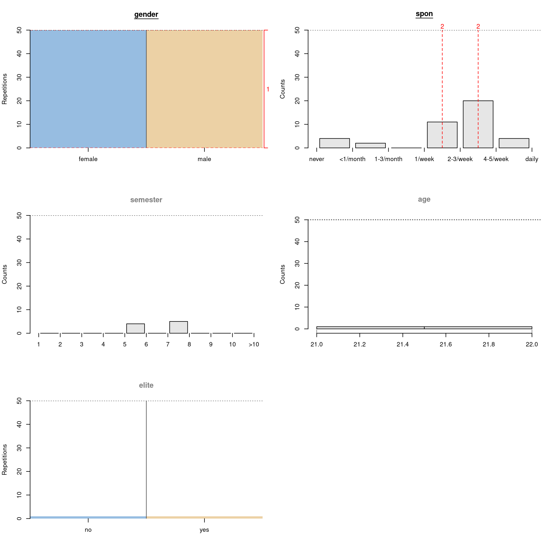
Regarding the variable gender, that is coded binarily here, there is only one possible cutpoint, which is used whenever the variable is used for splitting (including the first split in the original tree, as indicated in red). Looking at the ordered factor spon, we observe that a cutpoint between 2-3/week and 4-5/week occurred most frequently, followed by the neighboring cutpoint between 1/week and 2-3/week. These two cutpoints were also chosen in the original tree (as indicated by the red vertical lines; the number two indicates that this variable was used for the second split in each branch of the tree, cf. the illustration of the original tree. Other cutpoints only occurred very rarely. Finally, regarding the other variables semester, age, and elite (which were not selected in the original tree), we observe cutpoints between 5 and 8 for the variable semester, quite heterogenous cutpoints for the variable age, and the only possible cutpoint for the binary variable elite, that is used only in very few trees, as we saw above.
To conclude, the summary table and plots can help us gain some insight into the stability of our original Rasch tree by means of a resampling approach. Here, the DIF effects of gender and spon appear to be quite stable.
Acknowledgments
The work of Carolin Strobl was supported by grant STR1142/1-1 (“Methods to Account for Subject-Covariates in IRT-Models”) from the German Research Foundation (DFG). The work of Lennart Schneider was supported in part by grant 100019_152548 (“Detecting Heterogeneity in Complex IRT Models for Measuring Latent Traits”) from the Swiss National Science Foundation (SNF). The authors would like to thank the late Reinhold Hatzinger for important insights stimulated by conversations and the R package eRm Mair et al. (2020).
References
Chalmers, R. Philip. 2012. “mirt: A Multidimensional Item Response Theory Package for the R Environment.” Journal of Statistical Software 48 (6): 1–29. https://doi.org/10.18637/jss.v048.i06.
Chalmers, R. Philip. 2020. mirt: Multidimensional Item Response Theory. https://doi.org/10.32614/CRAN.package.mirt.
Mair, Patrick, and Reinhold Hatzinger. 2007. “Extended Rasch Modeling: The eRm Package for the Application of IRT Models in R.” Journal of Statistical Software 20 (9): 1–20. https://doi.org/10.18637/jss.v020.i09.
Mair, Patrick, Reinhold Hatzinger, and Marco Maier. 2020. eRm: Extended Rasch Modeling. https://doi.org/10.32614/CRAN.package.eRm.
Philipp, Michel, Achim Zeileis, and Carolin Strobl. 2016. “A Toolkit for Stability Assessment of Tree-Based Learners.” In Proceedings of COMPSTAT 2016 – 22nd International Conference on Computational Statistics, edited by Ana Colubi, Angela Blanco, and Cristian Gatu. The International Statistical Institute/International Association for Statistical Computing. https://www.zeileis.org/papers/Philipp+Zeileis+Strobl-2016.pdf.
Robitzsch, Alexander, Thomas Kiefer, and Margaret Wu. 2020. TAM: Test Analysis Modules. https://doi.org/10.32614/CRAN.package.TAM.
Strobl, C., J. Kopf, and A. Zeileis. 2015. “Rasch Trees: A New Method for Detecting Differential Item Functioning in the Rasch Model.” Psychometrika 80 (2): 289–316.
Trepte, S., and M. Verbeet, eds. 2010. Allgemeinbildung in Deutschland – Erkenntnisse aus dem SPIEGEL Studentenpisa-Test. VS Verlag. https://doi.org/10.1007/978-3-531-92543-1.
Zeileis, Achim, and Kurt Hornik. 2007. “Generalized M-Fluctuation Tests for Parameter Instability.” Statistica Neerlandica 61 (4): 488–508.
Zeileis, Achim, Torsten Hothorn, and Kurt Hornik. 2008. “Model-Based Recursive Partitioning.” Journal of Computational and Graphical Statistics 17 (2): 492–514.