zoo Quick Reference

This vignette gives a brief overview of (some of) the functionality contained in zoo including several nifty code snippets when dealing with (daily) financial data. It was originally written by Ajay Shah. For a more complete overview of the package’s functionality and extensibility see Zeileis and Grothendieck (2005, Journal of Statistical Software, doi:10.18637/jss.v014.i06). (contained as vignette("zoo", package = "zoo") in the package), the manual pages and the reference card.

Some of the examples below assume the availability of various data files which are all provided in the package. An easy way to make the available is to set the working directory as follows:

library("zoo")
setwd(file.path(system.file(package = "zoo"), "doc"))

Read a series from a text file

To read in data in a text file, read.table() and associated functions can be used as usual with zoo() being called subsequently. The convenience function read.zoo is a simple wrapper to these functions that assumes the index is in the first column of the file and the remaining columns are data.

Data in demo1.txt, where each row looks like

   23 Feb 2005|43.72

can be read in via

Sys.setlocale("LC_TIME", "C")

[1] "C"

inrusd <- read.zoo("demo1.txt", sep = "|", format="%d %b %Y")

The format argument causes the first column to be transformed to an index of class "Date". The Sys.setlocale is set to "C" here to assure that the English month abbreviations are read correctly. (It is unnecessary if the system is already set to a locale that understands English month abbreviations.)

The data in demo2.txt look like

   Daily,24 Feb 2005,2055.30,4337.00

and requires more attention because of the format of the first column.

tmp <- read.table("demo2.txt", sep = ",")
z <- zoo(tmp[, 3:4], as.Date(as.character(tmp[, 2]), format="%d %b %Y"))
colnames(z) <- c("Nifty", "Junior")

Query dates

To return all dates corresponding to a series index(z) or equivalently

time(z)

 [1] "2005-02-10" "2005-02-11" "2005-02-14" "2005-02-15" "2005-02-17"
 [6] "2005-02-18" "2005-02-21" "2005-02-22" "2005-02-23" "2005-02-24"
[11] "2005-02-25" "2005-02-28" "2005-03-01" "2005-03-02" "2005-03-03"
[16] "2005-03-04" "2005-03-07" "2005-03-08" "2005-03-09" "2005-03-10"

can be used. The first and last date can be obtained by

start(z)

[1] "2005-02-10"

end(inrusd)

[1] "2005-03-10"

Convert back into a plain matrix

To strip off the dates and just return a plain vector/matrix coredata can be used

plain <- coredata(z)
str(plain)

 num [1:20, 1:2] 2063 2082 2098 2090 2062 ...
 - attr(*, "dimnames")=List of 2
  ..$ : NULL
  ..$ : chr [1:2] "Nifty" "Junior"

Union and intersection

Unions and intersections of series can be computed by merge. The intersection are those days where both series have time points:

m <- merge(inrusd, z, all = FALSE)

whereas the union uses all dates and fills the gaps where one series has a time point but the other does not with NAs (by default):

m <- merge(inrusd, z)

cbind(inrusd, z) is almost equivalent to the merge call, but may lead to inferior naming in some situations hence merge is preferred

To combine a series with its lag, use

merge(inrusd, lag(inrusd, -1))

           inrusd lag(inrusd, -1)
2005-02-10  43.78              NA
2005-02-11  43.79           43.78
2005-02-14  43.72           43.79
2005-02-15  43.76           43.72
2005-02-16  43.82           43.76
2005-02-17  43.74           43.82
2005-02-18  43.84           43.74
2005-02-21  43.82           43.84
2005-02-22  43.72           43.82
2005-02-23  43.72           43.72
2005-02-24  43.70           43.72
2005-02-25  43.69           43.70
2005-02-28  43.64           43.69
2005-03-01  43.72           43.64
2005-03-02  43.70           43.72
2005-03-03  43.65           43.70
2005-03-04  43.71           43.65
2005-03-07  43.69           43.71
2005-03-09  43.67           43.69
2005-03-10  43.58           43.67

Visualization

By default, the plot() method generates a graph for each series in m

plot(m)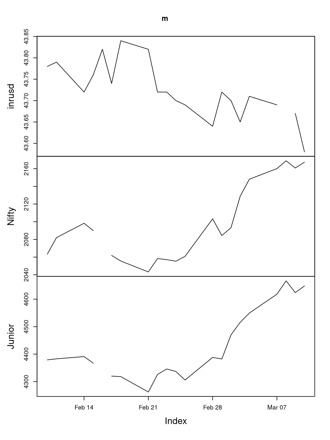

but several series can also be plotted in a single window.

plot(m[, 2:3], plot.type = "single", col = c("red", "blue"), lwd = 2)

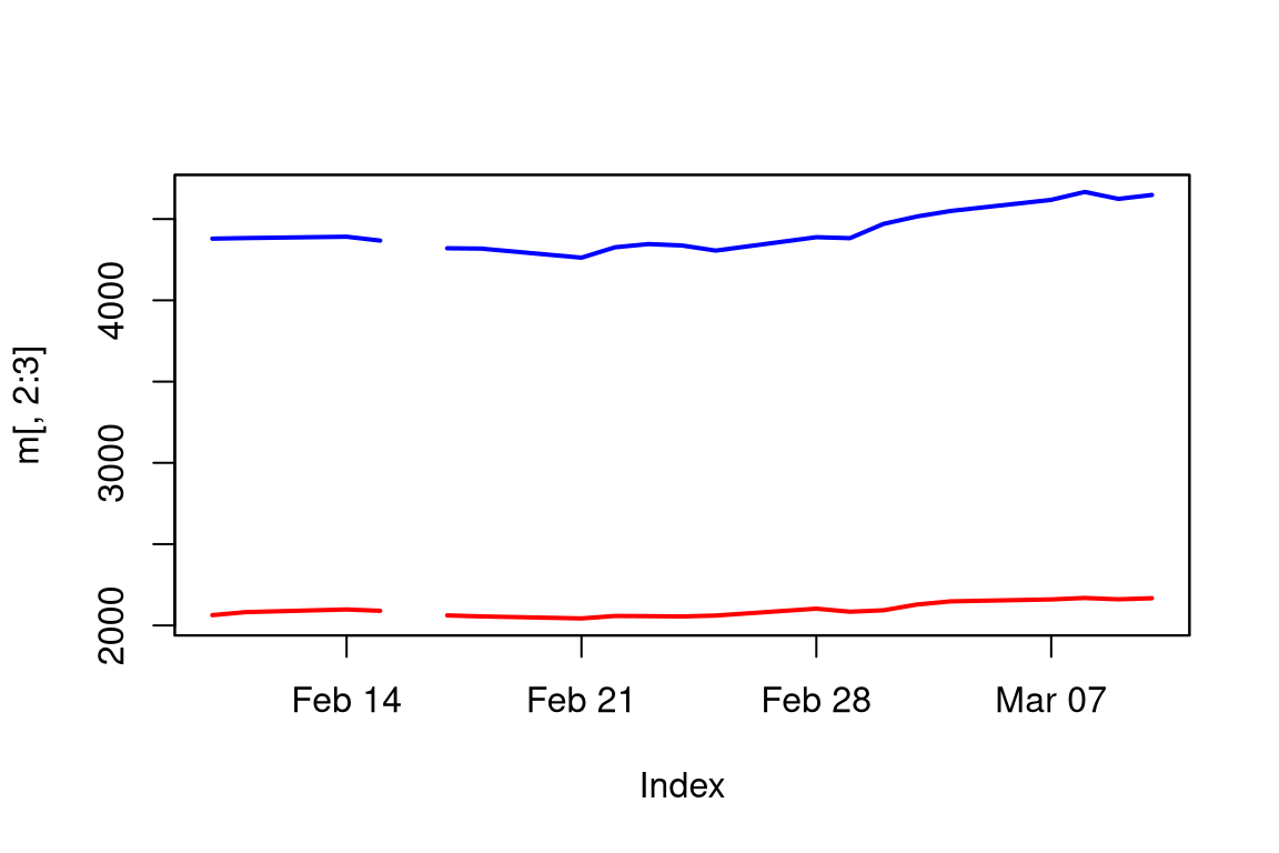
In addition to the plain base graphics plot() there are methods xyplot() for lattice, autoplot() for ggplot2, and tinyplot(). All of these provide many additional graphics capabilities, especially including facetting for multivariate series. For example, using the tinyplot package one can do:

library("tinyplot")
tinyplot(z, facet = Series ~ 1, theme = "clean2",
  palette = "Dark 3", lwd = 2, legend = FALSE)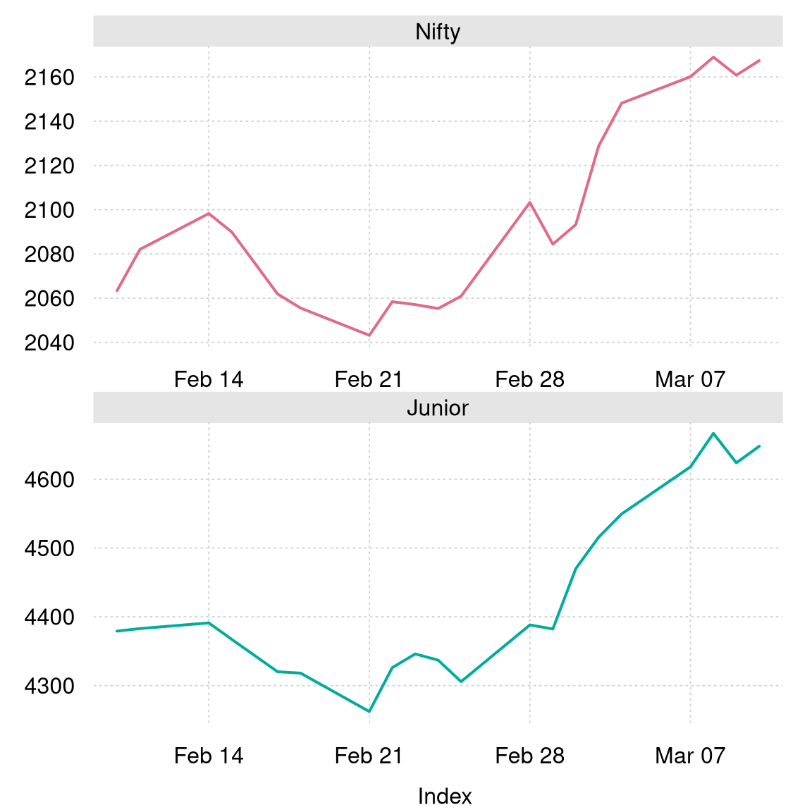

Select (a few) observations

Selections can be made for a range of dates of interest

window(z, start = as.Date("2005-02-15"), end = as.Date("2005-02-28"))

             Nifty  Junior
2005-02-15 2089.95 4367.25
2005-02-17 2061.90 4320.15
2005-02-18 2055.55 4318.15
2005-02-21 2043.20 4262.25
2005-02-22 2058.40 4326.10
2005-02-23 2057.10 4346.00
2005-02-24 2055.30 4337.00
2005-02-25 2060.90 4305.75
2005-02-28 2103.25 4388.20

and also just for a single date

m[as.Date("2005-03-10")]

           inrusd  Nifty  Junior
2005-03-10  43.58 2167.4 4648.05

Handle missing data

Various methods for dealing with NAs are available, including linear interpolation

interpolated <- na.approx(m)

`last observation carried forward’,

m <- na.locf(m)
m

           inrusd   Nifty  Junior
2005-02-10  43.78 2063.35 4379.20
2005-02-11  43.79 2082.05 4382.90
2005-02-14  43.72 2098.25 4391.15
2005-02-15  43.76 2089.95 4367.25
2005-02-16  43.82 2089.95 4367.25
2005-02-17  43.74 2061.90 4320.15
2005-02-18  43.84 2055.55 4318.15
2005-02-21  43.82 2043.20 4262.25
2005-02-22  43.72 2058.40 4326.10
2005-02-23  43.72 2057.10 4346.00
2005-02-24  43.70 2055.30 4337.00
2005-02-25  43.69 2060.90 4305.75
2005-02-28  43.64 2103.25 4388.20
2005-03-01  43.72 2084.40 4382.25
2005-03-02  43.70 2093.25 4470.00
2005-03-03  43.65 2128.85 4515.80
2005-03-04  43.71 2148.15 4549.55
2005-03-07  43.69 2160.10 4618.05
2005-03-08  43.69 2168.95 4666.70
2005-03-09  43.67 2160.80 4623.85
2005-03-10  43.58 2167.40 4648.05

and others.

Prices and returns

To compute log-difference returns in %, the following convenience function is defined

prices2returns <- function(x) 100*diff(log(x))

which can be used to convert all columns (of prices) into returns.

r <- prices2returns(m)

A 10-day rolling window standard deviations (for all columns) can be computed by

rollapply(r, 10, sd)

               inrusd     Nifty    Junior
2005-02-17 0.14599121 0.6993355 0.7878843
2005-02-18 0.14527421 0.6300543 0.8083622
2005-02-21 0.14115862 0.8949318 1.0412806
2005-02-22 0.15166883 0.9345299 1.0256508
2005-02-23 0.14285470 0.9454103 1.1957959
2005-02-24 0.13607992 0.9453855 1.1210963
2005-02-25 0.11962991 0.9334899 1.1105966
2005-02-28 0.11963193 0.8585071 0.9388661
2005-03-01 0.09716262 0.8569891 0.9131822
2005-03-02 0.09787943 0.8860388 1.0566389
2005-03-03 0.11568119 0.8659890 1.0176645

To go from a daily series to the series of just the last-traded-day of each month aggregate can be used

prices2returns(aggregate(m, as.yearmon, tail, 1))

             inrusd    Nifty   Junior
Mar 2005 -0.1375831 3.004453 5.752866

Analogously, the series can be aggregated to the last-traded-day of each week employing a convenience function nextfri that computes for each "Date" the next friday.

nextfri <- function(x) 7 * ceiling(as.numeric(x-5+4) / 7) + as.Date(5-4)
prices2returns(aggregate(na.locf(m), nextfri, tail, 1))

                inrusd      Nifty     Junior
2005-02-18  0.11411618 -1.2809533 -1.4883536
2005-02-25 -0.34273997  0.2599329 -0.2875731
2005-03-04  0.04576659  4.1464226  5.5076988
2005-03-11 -0.29785794  0.8921286  2.1419450

Here is a similar example of aggregate where we define to4sec analogously to nextfri in order to aggregate the zoo object zsec every 4 seconds.

zsec <- structure(1:10, index = structure(c(1234760403.968, 1234760403.969, 
1234760403.969, 1234760405.029, 1234760405.029, 1234760405.03, 
1234760405.03, 1234760405.072, 1234760405.073, 1234760405.073
), class = c("POSIXt", "POSIXct"), tzone = ""), class = "zoo")

to4sec <- function(x) as.POSIXct(4*ceiling(as.numeric(x)/4), origin = "1970-01-01")
aggregate(zsec, to4sec, tail, 1)

2009-02-16 05:00:04 2009-02-16 05:00:08 
                  3                  10 

Here is another example using the same zsec zoo object but this time rather than aggregating we truncate times to the second using the last data value for each such second. For large objects this will be much faster than using aggregate.zoo .

# tmp is zsec with time discretized into one second bins
tmp <- zsec
st <- start(tmp)
Epoch <- st - as.numeric(st)
time(tmp) <- as.integer(time(tmp) + 1e-7) + Epoch

# find index of last value in each one second interval
ix <- !duplicated(time(tmp), fromLast = TRUE)

# merge with grid 
merge(tmp[ix], zoo(, seq(start(tmp), end(tmp), "sec")))

2009-02-16 05:00:03 2009-02-16 05:00:04 2009-02-16 05:00:05 
                  3                  NA                  10 

# Here is a function which generalizes the above:

intraday.discretise <- function(b, Nsec) {
 st <- start(b)
 time(b) <- Nsec * as.integer(time(b)+1e-7) %/% Nsec + st -
 as.numeric(st)
 ix <- !duplicated(time(b), fromLast = TRUE)
 merge(b[ix], zoo(, seq(start(b), end(b), paste(Nsec, "sec"))))
}

intraday.discretise(zsec, 1)

2009-02-16 05:00:03 2009-02-16 05:00:04 2009-02-16 05:00:05 
                  3                  NA                  10 

Query Yahoo! Finance

When connected to the internet, Yahoo! Finance can be easily queried using the get.hist.quote function in

library("tseries")

if(online) {
  msft <- get.hist.quote(instrument = "MSFT", start = "2004-01-01", end = "2004-12-31")
  msft2 <- get.hist.quote(instrument = "MSFT", start = "2004-01-01", end = "2004-12-31",
    compression = "m", quote = "Close")
  save(msft, msft2, file = "msft2004.rda")
} else {
  load("msft2004.rda")
}

From version 0.9-30 on, get.hist.quote by default returns "zoo" series with a "Date" attribute (in previous versions these had to be transformed from "ts" `by hand’).

A daily series can be obtained by:

msft <- get.hist.quote(instrument = "MSFT", start = "2004-01-01", end = "2004-12-31")

A monthly series can be obtained and transformed by

msft2 <- get.hist.quote(instrument = "MSFT", start = "2004-01-01", end = "2004-12-31",
  compression = "m", quote = "Close")

Here, "yearmon" dates might be even more useful:

time(msft2) <- as.yearmon(time(msft2))

The same series can equivalently be computed from the daily series via

msft3 <- aggregate(msft[, "Close"], as.yearmon, tail, 1)

The corresponding returns can be computed via

r <- prices2returns(msft3)

where r is still a "zoo" series.

Summaries

Here we create a daily series and then find the series of quarterly means and standard deviations and also for weekly means and standard deviations where we define weeks to end on Tuesay.

We do the above separately for mean and standard deviation, binding the two results together and then show a different approach in which we define a custom ag function that can accept multiple function names as a vector argument.

date1 <- seq(as.Date("2001-01-01"), as.Date("2002-12-1"), by = "day")
len1 <- length(date1)
set.seed(1) # to make it reproducible
data1 <- zoo(rnorm(len1), date1)

# quarterly summary

data1q.mean <- aggregate(data1, as.yearqtr, mean)
data1q.sd <- aggregate(data1, as.yearqtr, sd)
head(cbind(mean = data1q.mean, sd = data1q.sd), main = "Quarterly")

                mean        sd
2001 Q1  0.108503596 0.8861821
2001 Q2 -0.006836172 0.9800027
2001 Q3 -0.042260559 0.9954100
2001 Q4  0.096188411 1.0336234
2002 Q1 -0.092684201 1.0337850
2002 Q2  0.049217429 1.0860119

# weekly summary - week ends on tuesday

# Given a date find the next Tuesday.
# Based on formula in Prices and Returns section.
nexttue <- function(x) 7 * ceiling(as.numeric(x - 2 + 4)/7) + as.Date(2 - 4)

data1w <- cbind(
       mean = aggregate(data1, nexttue, mean),
       sd = aggregate(data1, nexttue, sd)
)
head(data1w)

                  mean        sd
2001-01-02 -0.22140524 0.5728252
2001-01-09  0.29574667 0.8686111
2001-01-16 -0.02281531 1.2305420
2001-01-23  0.58834959 0.3993624
2001-01-30 -0.44463015 0.9619139
2001-02-06 -0.08522653 0.8349544

### ALTERNATIVE ###

# Create function ag like aggregate but takes vector of
# function names.

FUNs <- c(mean, sd)
ag <- function(z, by, FUNs) {
       f <- function(f) aggregate(z, by, f)
       do.call(cbind, sapply(FUNs, f, simplify = FALSE))
}

data1q <- ag(data1, as.yearqtr, c("mean", "sd"))
data1w <- ag(data1, nexttue, c("mean", "sd"))

head(data1q)

                mean        sd
2001 Q1  0.108503596 0.8861821
2001 Q2 -0.006836172 0.9800027
2001 Q3 -0.042260559 0.9954100
2001 Q4  0.096188411 1.0336234
2002 Q1 -0.092684201 1.0337850
2002 Q2  0.049217429 1.0860119

head(data1w)

                  mean        sd
2001-01-02 -0.22140524 0.5728252
2001-01-09  0.29574667 0.8686111
2001-01-16 -0.02281531 1.2305420
2001-01-23  0.58834959 0.3993624
2001-01-30 -0.44463015 0.9619139
2001-02-06 -0.08522653 0.8349544

A convenience function which can determine for a vector of "Date" observations whether it is a weekend or not

is.weekend <- function(x) ((as.numeric(x)-2) %% 7) < 2

The function is.weekend introduced above exploits the fact that a "Date" is essentially the number of days since 1970-01-01, a Thursday. A more intelligible function which yields identical results could be based on the "POSIXlt" class

is.weekend <- function(x) {
  x <- as.POSIXlt(x)
  x$wday > 5 | x$wday < 1
}