Fit a univariate generalized logisitc distribution (Type I: skew-logistic with location, scale, and shape parameters) to a sample of observations.
Usage
glogisfit(x, ...)
## Default S3 method:
glogisfit(x, weights = NULL, start = NULL, fixed = c(NA, NA, NA),
  method = "BFGS", hessian = TRUE, ...)
## S3 method for class 'formula'
glogisfit(formula, data, subset, na.action, weights, x = TRUE, ...)

## S3 method for class 'glogisfit'
plot(x, main = "", xlab = NULL, fill = "lightgray",
  col = "blue", lwd = 1, lty = 1, xlim = NULL, ylim = NULL,
  legend = "topright", moments = FALSE, ...)

## S3 method for class 'glogisfit'
summary(object, log = TRUE, breaks = NULL, ...)
## S3 method for class 'glogisfit'
coef(object, log = TRUE, ...)
## S3 method for class 'glogisfit'
vcov(object, log = TRUE, ...)
Arguments
x
a vector of observation (may be a ts or zoo time series).
weights
optional numeric vector of weights.
start
optional vector of starting values. The parametrization has to be in terms of location, log(scale), log(shape) where the original parameters (without logs) are as in dglogis. Default is to use c(0, 0, 0) (i.e., standard logistic). For details see below.
fixed
specification of fixed parameters (see description of start). NA signals that the corresponding parameter should be estimated. A standard logistic distribution could thus be fitted via fixed = c(NA, NA, 0).
method
character string specifying optimization method, see optim for the available options. Further options can be passed to optim through ….
hessian
logical. Should the Hessian be used to compute the variance/covariance matrix? If FALSE, no covariances or standard errors will be available in subsequent computations.
formula
symbolic description of the model, currently only x ~ 1 is supported.
data, subset, na.action
arguments controlling formula processing via model.frame.
main, xlab, fill, col, lwd, lty, xlim, ylim
standard graphical parameters, see plot and par.
legend
logical or character specification where to place a legend. legend = FALSE suppresses the legend. See legend for the character specification.
moments
logical. If a legend is produced, it can either show the parameter estimates (moments = FALSE, default) or the implied moments of the distribution.
object
a fitted glogisfit object.
log
logical option in some extractor methods indicating whether scale and shape parameters should be reported in logs (default) or the original levels.
breaks
interval breaks for the chi-squared goodness-of-fit test. Either a numeric vector of two or more cutpoints or a single number (greater than or equal to 2) giving the number of intervals.
…
arguments passed to methods.
Details
glogisfit estimates the generalized logistic distribution (Type I: skew-logistic) as given by dglogis. Optimization is performed numerically by optim using analytical gradients. For obtaining numerically more stable results the scale and shape parameters are specified in logs. Starting values are chosen as c(0, 0, 0), i.e., corresponding to a standard (symmetric) logistic distribution. If these fail, better starting values are obtained by running a Nelder-Mead optimization on the original problem (without logs) first.
A large list of standard extractor methods is supplied to conveniently compute with the fitted objects, including methods to the generic functions print, summary, plot (reusing hist and lines), coef, vcov, logLik, residuals, and estfun and bread (from the sandwich package).
The methods for coef, vcov, summary, and bread report computations pertaining to the scale/shape parameters in logs by default, but allow for switching back to the original levels (employing the delta method).
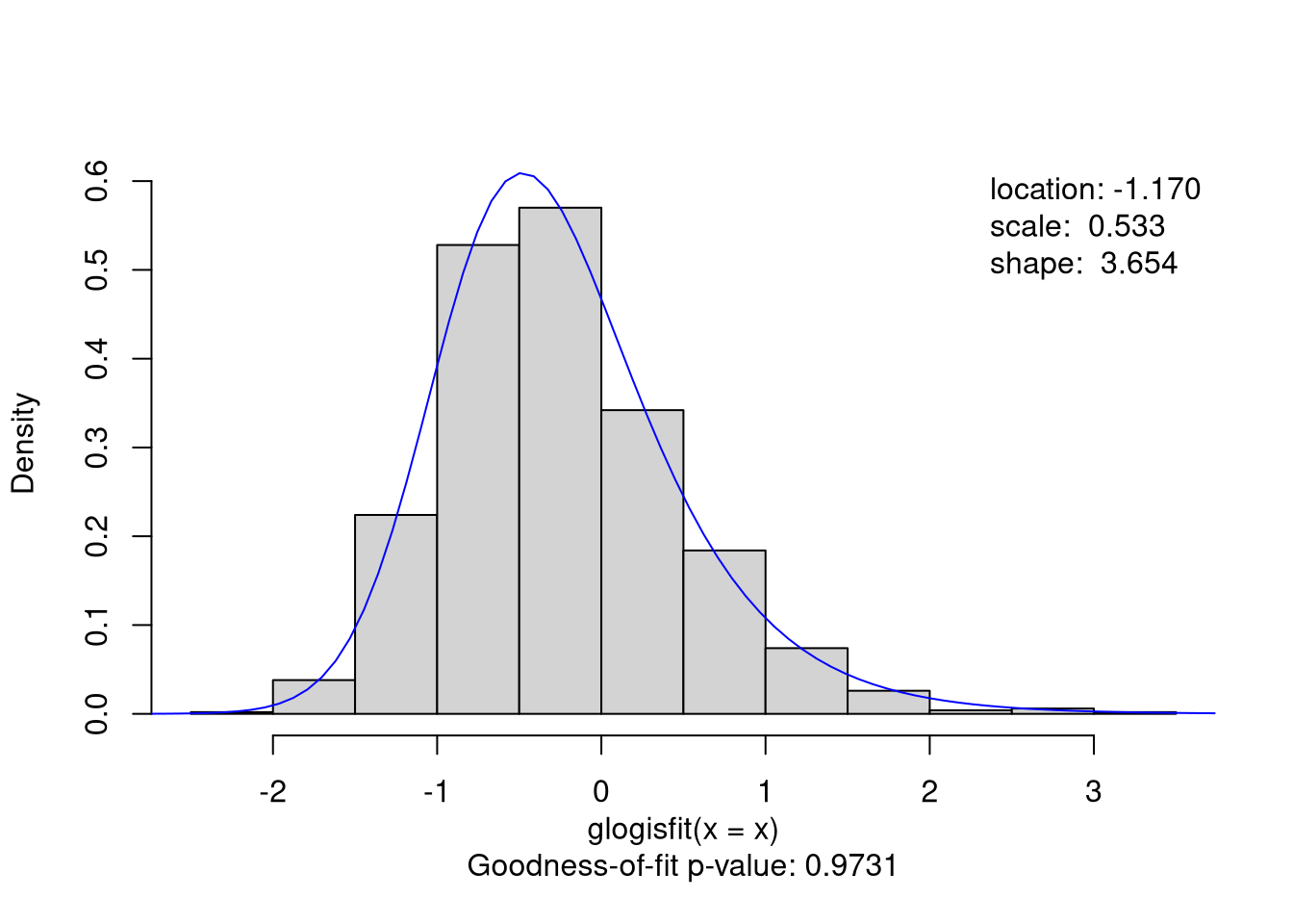
Visualization employs a histogramm of the original data along with lines for the estimated density.
Further structural change methods for “glogisfit” objects are described in breakpoints.glogisfit.
Value
glogisfit returns an object of class “glogisfit”, i.e., a list with components as follows.
coefficients
estimated parameters from the model (with scale/shape in logs, if included),
vcov
associated estimated covariance matrix,
loglik
log-likelihood of the fitted model,
df
number of estimated parameters,
n
number of observations,
nobs
number of observations with non-zero weights,
weights
the weights used (if any),
optim
output from the optim call for maximizing the log-likelihood,
method
the method argument passed to the optim call,
parameters
the full set of model parameters (location/scale/shape), including estimated and fixed parameters, all in original levels (without logs),
moments
associated mean/variance/skewness,
start
the starting values for the parameters passed to the optim call,
fixed
the original specification of fixed parameters,
call
the original function call,
x
the original data,
converged
logical indicating successful convergence of optim,
terms
the terms objects for the model (if the formula method was used).
References
Shao Q (2002). Maximum Likelihood Estimation for Generalised Logistic Distributions. Communications in Statistics – Theory and Methods, 31(10), 1687–1700.
Windberger T, Zeileis A (2014). Structural Breaks in Inflation Dynamics within the European Monetary Union. Eastern European Economics, 52(3), 66–88.