Harmonised Index of Consumer Prices (1990–2010, OECD)

Description

Time series data with HICP (Harmonised Index of Consumer Prices) for 21 countries (plus EU) for 1990–2010 as provided by the OECD; and corresponding seasonally adjusted inflation ratios.

Usage

  data("HICP")

  data("hicps")  

Format

Monthly multiple “zooreg” time series with “yearmon” index from Jan 1990 (HICP) or Feb 1990 (hicps) to Dec 2010 for 21 countries (plus EU).

Details

HICP contains the raw unadjusted Harmonised Index of Consumer Prices as provided by the OECD from which unadjusted inflation rates can be easily computed (see examples).

As the different countries have rather different seasonal patterns which vary over time (especially in the 2000s), they will typically require seasonal adjustment before modeling. Hence, a seasonally adjusted version of the inflation rate series is provided as hicps, where X-12-ARIMA (version 0.3) has been employed for adjusted. An alternative seasonal adjustment can be easily computed use stl (see examples).

Source

Organisation for Economic Co-operation and Development (OECD)

https://data-explorer.oecd.org/

References

Wikipedia (2010). "Harmonised Index of Consumer Prices – Wikipedia, The Free Encyclopedia." https://en.wikipedia.org/wiki/Harmonised_Index_of_Consumer_Prices, accessed 2010-06-10.

Windberger T, Zeileis A (2014). Structural Breaks in Inflation Dynamics within the European Monetary Union. Eastern European Economics, 52(3), 66–88.

Examples

library("glogis")

## price series
data("HICP", package = "glogis")

## corresponding raw unadjusted inflation rates (in percent)
hicp <- 100 * diff(log(HICP))

## seasonal adjustment of inflation rates (via STL)
hicps1 <- do.call("merge", lapply(1:ncol(hicp), function(i) {
  z <- na.omit(hicp[,i])
  coredata(z) <- coredata(as.ts(z) - stl(as.ts(z), s.window = 13)$time.series[, "seasonal"])
  z
}))
colnames(hicps1) <- colnames(hicp)

## load X-12-ARIMA adjusted inflation rates
data("hicps", package = "glogis")

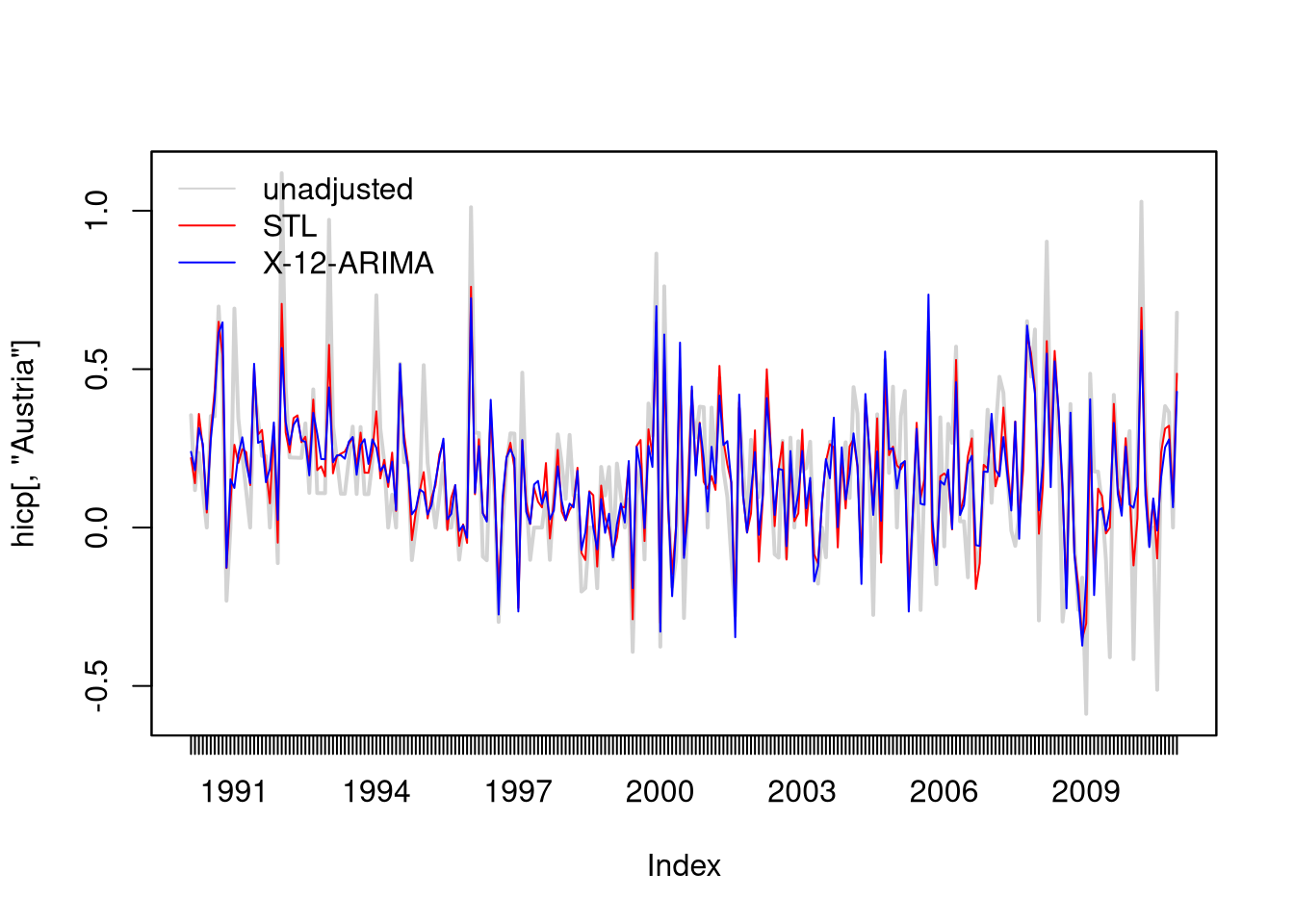
## compare graphically for one country (Austria)
plot(hicp[, "Austria"], lwd = 2, col = "lightgray")
lines(hicps1[, "Austria"], col = "red")
lines(hicps[, "Austria"], col = "blue")
legend("topleft", c("unadjusted", "STL", "X-12-ARIMA"), lty = c(1, 1, 1),
  col = c("lightgray", "red", "blue"), bty = "n")

## compare graphically across all countries (via lattice)
if(require("lattice")) {
trellis.par.set(theme = canonical.theme(color = FALSE))
xyplot(merge(hicp, hicps1, hicps), 
  screen = names(hicp)[rep(1:ncol(hicp), 3)],
  col = c("lightgray", "red", "blue")[rep(1:3, each = ncol(hicp))],
  lwd = c(2, 1, 1)[rep(1:3, each = ncol(hicp))])
}