Heteroscedastic Binary Response GLMs

Description

Fit heteroscedastic binary response models via maximum likelihood.

Usage

hetglm(formula, data, subset, na.action, weights, offset,
  family = binomial(link = "probit"),
  link.scale = c("log", "sqrt", "identity"),
  control = hetglm.control(...),
  model = TRUE, y = TRUE, x = FALSE, ...)

hetglm.fit(x, y, z = NULL, weights = NULL, offset = NULL,
  family = binomial(), link.scale = "log", control = hetglm.control())

Arguments

formula	symbolic description of the model (of type y ~ x or y ~ x | z; for details see below).
data, subset, na.action	arguments controlling formula processing via model.frame.
weights	optional numeric vector of case weights.
offset	optional numeric vector(s) with an a priori known component to be included in the linear predictor(s).
family	family object (including the link function of the mean model).
link.scale	character specification of the link function in the latent scale model.
control	a list of control arguments specified via hetglm.control.
model, y, x	logicals. If TRUE the corresponding components of the fit (model frame, response, model matrix) are returned. For hetglm.fit, x should be a numeric regressor matrix and y should be the numeric response vector (with values in (0,1)).
z	numeric matrix. Regressor matrix for the precision model, defaulting to an intercept only.
…	arguments passed to hetglm.control.

Details

A set of standard extractor functions for fitted model objects is available for objects of class “hetglm”, including methods to the generic functions print, summary, coef, vcov, logLik, residuals, predict, terms, update, model.frame, model.matrix, estfun and bread (from the sandwich package), and coeftest (from the lmtest package).

Value

hetglm returns an object of class “hetglm”, i.e., a list with components as follows. hetglm.fit returns an unclassed list with components up to converged.

coefficients	a list with elements “mean” and “scale” containing the coefficients from the respective models,
residuals	a vector of raw residuals (observed - fitted),
fitted.values	a vector of fitted means,
optim	output from the optim call for maximizing the log-likelihood,
method	the method argument passed to the optim call,
control	the control arguments passed to the optim call,
start	the starting values for the parameters passed to the optim call,
weights	the weights used (if any),
offset	the list of offset vectors used (if any),
n	number of observations,
nobs	number of observations with non-zero weights,
df.null	residual degrees of freedom in the homoscedastic null model,
df.residual	residual degrees of freedom in the fitted model,
loglik	log-likelihood of the fitted model,
loglik.null	log-likelihood of the homoscedastic null model,
dispersion	estimate of the dispersion parameter (if any),
vcov	covariance matrix of all parameters in the model,
family	the family object used,
link	a list with elements “mean” and “scale” containing the link objects for the respective models,
converged	logical indicating successful convergence of optim,
call	the original function call,
formula	the original formula,
terms	a list with elements “mean”, “scale” and “full” containing the terms objects for the respective models,
levels	a list with elements “mean”, “scale” and “full” containing the levels of the categorical regressors,
contrasts	a list with elements “mean” and “scale” containing the contrasts corresponding to levels from the respective models,
model	the full model frame (if model = TRUE),
y	the response vector (if y = TRUE),
x	a list with elements “mean” and “scale” containing the model matrices from the respective models (if x = TRUE).

See Also

Formula

Examples

library("glmx")

## Generate artifical binary data from a latent
## heteroscedastic normally distributed variable
set.seed(48)
n <- 200
x <- rnorm(n)
ystar <- 1 + x +  rnorm(n, sd = exp(x))
y  <- factor(ystar > 0) 

## visualization
par(mfrow = c(1, 2))
plot(ystar ~ x, main = "latent")
abline(h = 0, lty = 2)
plot(y ~ x, main = "observed")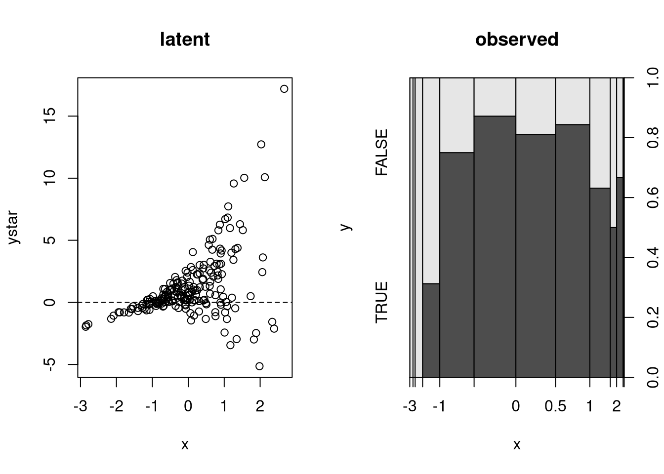

## model fitting of homoscedastic model (m0a/m0b)
## and heteroscedastic model (m)
m0a <- glm(y ~ x, family = binomial(link = "probit"))
m0b <- hetglm(y ~ x | 1)
m <- hetglm(y ~ x)

## coefficient estimates
cbind(heteroscedastic = coef(m),
  homoscedastic = c(coef(m0a), 0))

            heteroscedastic homoscedastic
(Intercept)        1.109258     0.5320893
x                  1.086656     0.3262606
(scale)_x          1.267372     0.0000000

## summary of correct heteroscedastic model
summary(m)

Call:
hetglm(formula = y ~ x)

Deviance residuals:
    Min      1Q  Median      3Q     Max 
-2.0380 -0.0022  0.5467  0.6974  1.5845 

Coefficients (binomial model with probit link):
            Estimate Std. Error z value Pr(>|z|)    
(Intercept)   1.1093     0.1401   7.918 2.42e-15 ***
x             1.0867     0.1492   7.284 3.24e-13 ***

Latent scale model coefficients (with log link):
  Estimate Std. Error z value Pr(>|z|)    
x   1.2674     0.2015   6.291 3.16e-10 ***
---
Signif. codes:  0 '***' 0.001 '**' 0.01 '*' 0.05 '.' 0.1 ' ' 1 

Log-likelihood: -92.92 on 3 Df
LR test for homoscedasticity: 46.14 on 1 Df, p-value: 1.101e-11
Dispersion: 1
Number of iterations in nlminb optimization: 9 

## Generate artificial binary data with a single binary regressor
## driving the heteroscedasticity in a model with two regressors
set.seed(48)
n <- 200
x <- rnorm(n)
z <- rnorm(n)
a <- factor(sample(1:2, n, replace = TRUE))
ystar <- 1 + c(0, 1)[a] + x + z + rnorm(n, sd = c(1, 2)[a])
y  <- factor(ystar > 0) 

## fit "true" heteroscedastic model
m1 <- hetglm(y ~ a + x + z | a)

## fit interaction model
m2 <- hetglm(y ~ a/(x + z) | 1)

## although not obvious at first sight, the two models are
## nested. m1 is a restricted version of m2 where the following
## holds: a1:x/a2:x == a1:z/a2:z
if(require("lmtest")) lrtest(m1, m2)

Likelihood ratio test

Model 1: y ~ a + x + z | a
Model 2: y ~ a/(x + z) | 1
  #Df  LogLik Df  Chisq Pr(>Chisq)
1   5 -75.088                     
2   6 -75.064  1 0.0466     0.8292

## both ratios are == 2 in the data generating process
c(x = coef(m2)[3]/coef(m2)[4], z = coef(m2)[5]/coef(m2)[6])

  x.a1:x   z.a1:z 
3.758025 3.179625 

if(require("AER")) {

## Labor force participation example from Greene
## (5th edition: Table 21.3, p. 682)
## (6th edition: Table 23.4, p. 790)

## data (including transformations)
data("PSID1976", package = "AER")
PSID1976$kids <- with(PSID1976, factor((youngkids + oldkids) > 0,
  levels = c(FALSE, TRUE), labels = c("no", "yes")))
PSID1976$fincome <- PSID1976$fincome/10000

## Standard probit model via glm()
lfp0a <- glm(participation ~ age + I(age^2) + fincome + education + kids,
  data = PSID1976, family = binomial(link = "probit"))

## Standard probit model via hetglm() with constant scale
lfp0b <- hetglm(participation ~ age + I(age^2) + fincome + education + kids | 1,
  data = PSID1976)

## Probit model with varying scale
lfp1 <- hetglm(participation ~ age + I(age^2) + fincome + education + kids | kids + fincome,
  data = PSID1976)

## Likelihood ratio and Wald test
lrtest(lfp0b, lfp1)
waldtest(lfp0b, lfp1)

## confusion matrices
table(true = PSID1976$participation,
  predicted = fitted(lfp0b) <= 0.5)
table(true = PSID1976$participation,
  predicted = fitted(lfp1) <= 0.5)



## Adapted (and somewhat artificial) example to illustrate that
## certain models with heteroscedastic scale can equivalently
## be interpreted as homoscedastic scale models with interaction
## effects.

## probit model with main effects and heteroscedastic scale in two groups
m <- hetglm(participation ~ kids + fincome | kids, data = PSID1976)

## probit model with interaction effects and homoscedastic scale
p <- glm(participation ~ kids * fincome, data = PSID1976,
   family = binomial(link = "probit"))

## both likelihoods are equivalent
logLik(m)
logLik(p)

## intercept/slope for the kids=="no" group
coef(m)[c(1, 3)]
coef(p)[c(1, 3)]

## intercept/slope for the kids=="yes" group
c(sum(coef(m)[1:2]), coef(m)[3]) / exp(coef(m)[4])
coef(p)[c(1, 3)] + coef(p)[c(2, 4)]

## Wald tests for the heteroscedasticity effect in m and the 
## interaction effect in p are very similar
coeftest(m)[4,]
coeftest(p)[4,]

## corresponding likelihood ratio tests are equivalent
## (due to the invariance of the MLE)
m0 <- hetglm(participation ~ kids + fincome | 1, data = PSID1976)
p0 <- glm(participation ~ kids + fincome, data = PSID1976,
  family = binomial(link = "probit"))
lrtest(m0, m)
lrtest(p0, p)

}

Likelihood ratio test

Model 1: participation ~ kids + fincome
Model 2: participation ~ kids * fincome
  #Df  LogLik Df  Chisq Pr(>Chisq)
1   3 -510.65                     
2   4 -510.10  1 1.0947     0.2954