Exchange Rate Regime Analysis for the Indian Rupee
We investigate the Indian exchange rate regime starting from 1993 when trading in the Indian rupee began up to the end of 2007. This reproduces the analysis from Zeileis et al. (2010) which includes a more detailed discussion.
Analysis
Exchange rate regime analysis is based on a linear regression model for cross-currency returns. A large data set derived from exchange rates available online from the US Federal Reserve at https://www.federalreserve.gov/releases/h10/Hist/ is provided in the FXRatesCHF data set in fxregime.
It is a zoo series containing 25 daily time series from 1971-01-04 to 2010-02-12. The columns correspond to the prices for various currencies (in ISO 4217 format) with respect to CHF as the unit currency.
India is an expanding economy with a currency that has been receiving increased interest over the last years. India is in the process of evolving away from a closed economy towards a greater integration with the world on both the current account and the capital account. This has brought considerable stress upon the pegged exchange rate regime. Therefore, we try to track the evolution of the INR exchange rate regime since trading in the INR began in about 1993 up to the end of 2007. The currency basket employed consists of the most important floating currencies (USD, JPY, EUR, GBP). Because EUR can only be used for the time after its introduction as official euro-zone currency in 1999, we employ the exchange rates of the German mark (DEM, the most important currency in the EUR zone) adjusted to EUR rates. The combined returns are denoted DUR below in FXRatesCHF:
Weekly rather than daily returns are employed to reduce the noise in the data and alleviate the computational burden of the dating algorithm of order \(O(n^2)\).
Using the full sample, we establish a single exchange rate regression only to show that there is not a single stable regime and to gain some exploratory insights from the associated fluctuation process.
inr_lm <- fxlm(INR ~ USD + JPY + DUR + GBP, data = inr)As we do not expect to be able to draw valid conclusions from the coefficients of a single regression, we do not report the coefficients and rather move on directly to assessing its stability using the associated empirical fluctuation process.
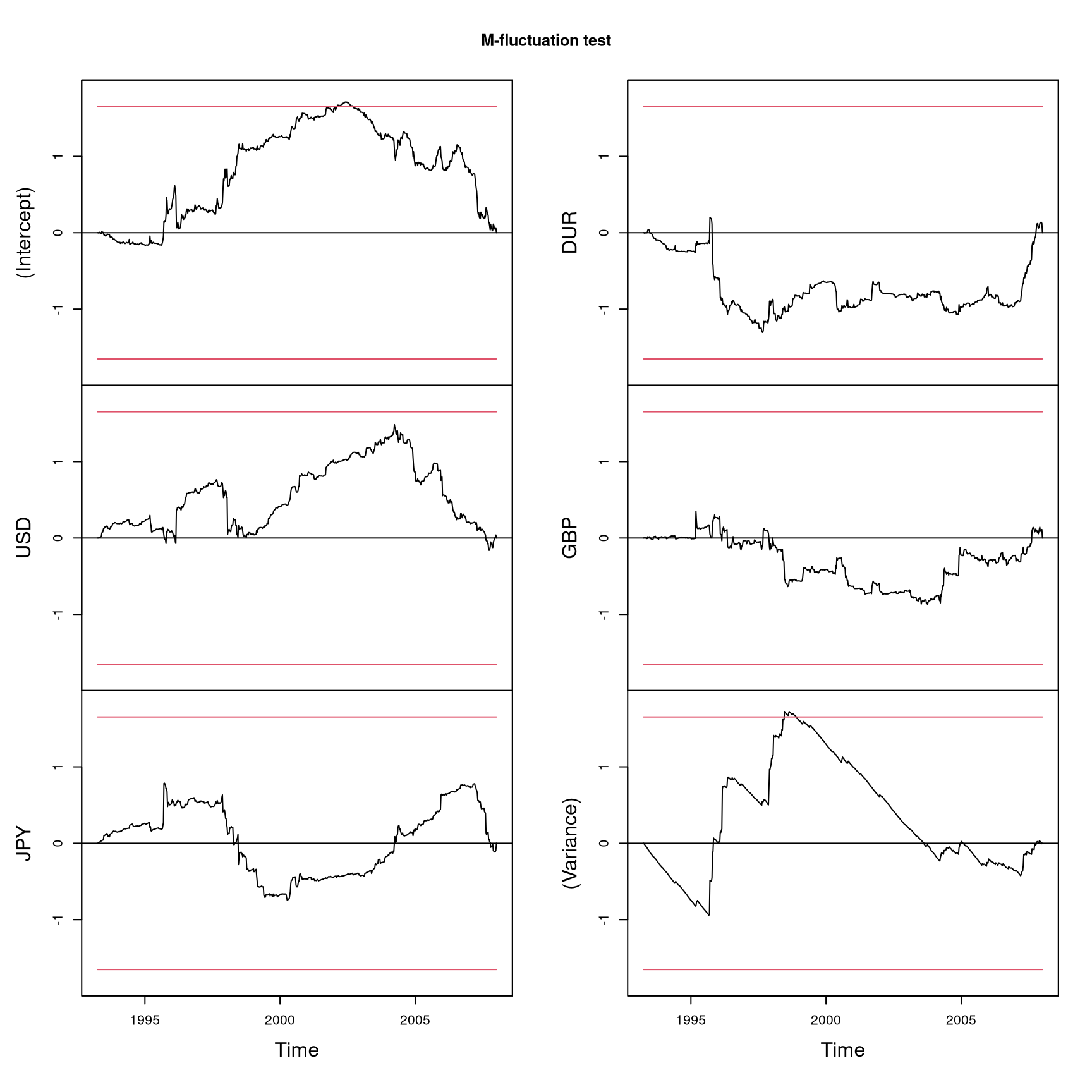
This shows that there is significant instability because two processes (intercept and variance) exceed their 5% level boundaries. More formally, the corresponding double maximum can be performed by
sctest(inr_efp)
##
##  M-fluctuation test
##
## data:  inr_efp
## f(efp) = 1.7242, p-value = 0.03099
This \(p\)~value is not very small because there seem to be several changes in various parameters. A more suitable test in such a situation would be the Nyblom–Hansen test
sctest(inr_efp, functional = meanL2BB)
##
##  M-fluctuation test
##
## data:  inr_efp
## f(efp) = 3.1147, p-value = 0.005
However, the multivariate fluctuation process is interesting as a visualization of the changes in the different parameters. The process for the variance \(\sigma^2\) has the most distinctive shape revealing at least four different regimes: at first, a variance that is lower than the overall average (and hence a decreasing process), then a much larger variance (up to the boundary crossing), a much smaller variance again and finally a period where the variance is roughly the full-sample average. Other interesting processes are the intercept and maybe the USD and DUR. The latter two are not significant but have some peaks revealing a decrease and increase, respectively, in the corresponding coefficients.
To capture this exploratory assessment in a formal way, a dating procedure is conducted for \(1, \dots, 10\) breaks and a minimal segment size of \(20\) observations.
inr_reg <- fxregimes(INR ~ USD + JPY + DUR + GBP,
  data = inr, h = 20, breaks = 10)
## [1] TRUEThe associated segmented negative log-likelihood (NLL) and LWZ criterion. Both can be visualized via
plot(inr_reg)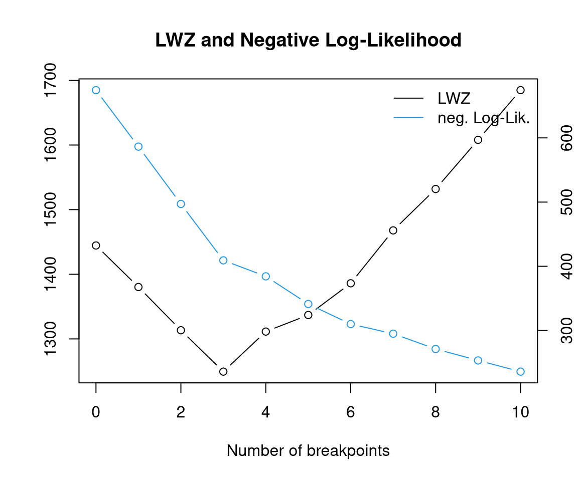
NLL is decreasing quickly up to \(3\) breaks with a kink in the slope afterwards. Similarly, LWZ takes its minimum for \(3\) breaks, choosing a 4-segment model. The confidence intervals corresponding to the breaks can be obtained by
confint(inr_reg, level = 0.9)
##
##   Confidence intervals for breakpoints
##   of optimal 4-segment partition:
##
## Call:
## confint.fxregimes(object = inr_reg, level = 0.9)
##
## Breakpoints at observation number:
##   5 % breakpoints 95 %
## 1  84         100  101
## 2 280         281  298
## 3 556         572  574
##
## Corresponding to breakdates:
##          5 % breakpoints       95 %
## 1 1994-11-11  1995-03-03 1995-03-10
## 2 1998-08-14  1998-08-21 1998-12-18
## 3 2003-11-28  2004-03-19 2004-04-02
showing that the start/end of segments with low variance can be determined more precisely than for segments with high variance.
The parameter estimates for all segments can be queried via
coef(inr_reg)
##                         (Intercept)       USD         JPY         DUR
## 1993-04-09--1995-03-03 -0.005740591 0.9716100 0.023466575  0.01126713
## 1995-03-10--1998-08-21  0.161133317 0.9431395 0.066918732 -0.02606616
## 1998-08-28--2004-03-19  0.018610654 0.9933245 0.009763423  0.09831871
## 2004-03-26--2008-01-04 -0.057614447 0.7464939 0.125614049  0.43544995
##                                 GBP (Variance)
## 1993-04-09--1995-03-03  0.020370927 0.02476617
## 1995-03-10--1998-08-21  0.042358762 0.85392476
## 1998-08-28--2004-03-19 -0.003220436 0.07554646
## 2004-03-26--2008-01-04  0.121368661 0.33473933
The most striking observation from the segmented coefficients is that INR was closely pegged to USD up to 2004-03-19 when it shifted to a basket peg in which USD has still the highest weight but considerably less than before. Furthermore, the changes in \(\sigma\) are remarkable, roughly matching the exploratory observations from the empirical fluctuation process. A more detailed look at the full summaries provided below shows that the first period is a clear and tight USD peg. During that time, pressure to appreciate was blocked by purchases of USD by the central bank. The second period, including the time of the East Asian crisis, saw a highly increased flexibility in the exchange rates. Although the Reserve Bank of India (RBI) made public statements about managing volatility on the currency market, the credibility of these statements were low in the eyes of the market. The third period exposes much tighter pegging again with low volatility, some appreciation and some small (but significant) weight on DUR. In the fourth period after March 2004, India moved away from the tight USD peg to a basket peg involving several currencies with greater flexibility (but smaller than in the second period). In this period, reserves in excess of 20% of GDP were held by the RBI, and a modest pace of reserves accumulation has continued.
inr_rf <- refit(inr_reg)
lapply(inr_rf, summary)
## $`1993-04-09--1995-03-03`
##
## Call:
## fxlm(formula = object$formula, data = window(object$data, start = sbp[i],
##     end = ebp[i]))
##
## Residuals:
##      Min       1Q   Median       3Q      Max
## -0.89169 -0.03021  0.00528  0.03859  0.89131
##
## Coefficients:
##              Estimate Std. Error t value Pr(>|t|)
## (Intercept) -0.005741   0.016507  -0.348   0.7288
## USD          0.971610   0.017626  55.124   <2e-16 ***
## JPY          0.023467   0.013988   1.678   0.0967 .
## DUR          0.011267   0.032338   0.348   0.7283
## GBP          0.020371   0.024284   0.839   0.4037
## ---
## Signif. codes:  0 '***' 0.001 '**' 0.01 '*' 0.05 '.' 0.1 ' ' 1
##
## Residual standard error: 0.1615 on 95 degrees of freedom
## Multiple R-squared:  0.9893, Adjusted R-squared:  0.9889
## F-statistic:  2205 on 4 and 95 DF,  p-value: < 2.2e-16
##
##
## $`1995-03-10--1998-08-21`
##
## Call:
## fxlm(formula = object$formula, data = window(object$data, start = sbp[i],
##     end = ebp[i]))
##
## Residuals:
##     Min      1Q  Median      3Q     Max
## -4.8702 -0.2943 -0.1225  0.2002  4.5560
##
## Coefficients:
##             Estimate Std. Error t value Pr(>|t|)
## (Intercept)  0.16113    0.07052   2.285   0.0235 *
## USD          0.94314    0.07372  12.794   <2e-16 ***
## JPY          0.06692    0.04813   1.390   0.1662
## DUR         -0.02607    0.15530  -0.168   0.8669
## GBP          0.04236    0.07980   0.531   0.5962
## ---
## Signif. codes:  0 '***' 0.001 '**' 0.01 '*' 0.05 '.' 0.1 ' ' 1
##
## Residual standard error: 0.9371 on 176 degrees of freedom
## Multiple R-squared:  0.7289, Adjusted R-squared:  0.7227
## F-statistic: 118.3 on 4 and 176 DF,  p-value: < 2.2e-16
##
##
## $`1998-08-28--2004-03-19`
##
## Call:
## fxlm(formula = object$formula, data = window(object$data, start = sbp[i],
##     end = ebp[i]))
##
## Residuals:
##      Min       1Q   Median       3Q      Max
## -0.94397 -0.12781 -0.02506  0.08499  1.11702
##
## Coefficients:
##              Estimate Std. Error t value Pr(>|t|)
## (Intercept)  0.018611   0.016292   1.142  0.25427
## USD          0.993324   0.016092  61.726  < 2e-16 ***
## JPY          0.009763   0.009838   0.992  0.32185
## DUR          0.098319   0.033850   2.905  0.00397 **
## GBP         -0.003220   0.020529  -0.157  0.87546
## ---
## Signif. codes:  0 '***' 0.001 '**' 0.01 '*' 0.05 '.' 0.1 ' ' 1
##
## Residual standard error: 0.2772 on 286 degrees of freedom
## Multiple R-squared:  0.9688, Adjusted R-squared:  0.9684
## F-statistic:  2222 on 4 and 286 DF,  p-value: < 2.2e-16
##
##
## $`2004-03-26--2008-01-04`
##
## Call:
## fxlm(formula = object$formula, data = window(object$data, start = sbp[i],
##     end = ebp[i]))
##
## Residuals:
##      Min       1Q   Median       3Q      Max
## -2.19182 -0.29861  0.01349  0.25854  1.57820
##
## Coefficients:
##             Estimate Std. Error t value Pr(>|t|)
## (Intercept) -0.05761    0.04195  -1.373 0.171227
## USD          0.74649    0.04458  16.746  < 2e-16 ***
## JPY          0.12561    0.04230   2.970 0.003361 **
## DUR          0.43545    0.11588   3.758 0.000227 ***
## GBP          0.12137    0.05608   2.164 0.031673 *
## ---
## Signif. codes:  0 '***' 0.001 '**' 0.01 '*' 0.05 '.' 0.1 ' ' 1
##
## Residual standard error: 0.586 on 193 degrees of freedom
## Multiple R-squared:  0.8002, Adjusted R-squared:  0.796
## F-statistic: 193.2 on 4 and 193 DF,  p-value: < 2.2e-16
Summary
For the Indian rupee, a 4-segment model is found with a close linkage of INR to USD in the first three periods (with tight/flexible/tight pegging, respectively) before moving to a more flexible basket peg in spring 2004.
The existing literature classifies the INR is a de facto pegged exchange rate to the USD in the period after April 1993. The results above show the fine structure of this pegged exchange rate; it supplies dates demarcating the four phases of the exchange rate regime; and it finds that by the fourth period, there was a basket peg in operation.