Exchange Rate Regime Analysis for the Chinese Yuan
Analysis
Exchange rate regime analysis is based on a linear regression model for cross-currency returns. A large data set derived from exchange rates available online from the US Federal Reserve at https://www.federalreserve.gov/releases/h10/Hist/ is provided in the FXRatesCHF data set in fxregime.
It is a zoo series containing 25 daily time series from 1971-01-04 to 2010-02-12. The columns correspond to the prices for various currencies (in ISO 4217 format) with respect to CHF as the unit currency.
In the following, we investigate the exchange rate regime for the Chinese yuan CNY which was fixed to the US dollar USD in the years leading up to mid-2005. In July 2005, China announced a small appreciation of CNY, and, in addition, a reform of the exchange rate regime. The People’s Bank of China (PBC) announced this reform to involve a shift away from the fixed exchange rate to a basket of currencies with greater flexibility. In August 2005, PBC also announced that USD, JPY, EUR and KRW would be the currencies in this basket. Further currencies announced to be of interest are GBP, MYR, SGD, RUB, AUD, THB and CAD.
Despite the announcements of the PBC, little evidence could be found for China moving away from a USD peg in the months after July 2005 (Shah et al. 2005). To begin our investigation here, we follow up on our own analysis from autumn 2005: Using daily returns for the first three months after the announcement, we establish a stable exchange regression and monitor it in the subsequent months. The currencies considered by Zeileis et al. (2010) are a basket of the most important floating currencies (USD, JPY, EUR, GBP). The returns can be extracted from FXRatesCHF and pre-processed via
In a first step, we fit the exchange regression for these first three months after the announcements of the PBC.
cny_lm <- fxlm(CNY ~ USD + JPY + EUR + GBP,
  data = window(cny, end = as.Date("2005-10-31")))
summary(cny_lm)
##
## Call:
## fxlm(formula = CNY ~ USD + JPY + EUR + GBP, data = window(cny,
##     end = as.Date("2005-10-31")))
##
## Residuals:
##       Min        1Q    Median        3Q       Max
## -0.065697 -0.021036  0.001147  0.021440  0.069985
##
## Coefficients:
##              Estimate Std. Error t value Pr(>|t|)
## (Intercept) -0.004782   0.003688  -1.297    0.199
## USD          0.999653   0.008779 113.868   <2e-16 ***
## JPY          0.004668   0.010669   0.437    0.663
## EUR         -0.014238   0.026516  -0.537    0.593
## GBP         -0.007744   0.014568  -0.532    0.597
## ---
## Signif. codes:  0 '***' 0.001 '**' 0.01 '*' 0.05 '.' 0.1 ' ' 1
##
## Residual standard error: 0.02953 on 63 degrees of freedom
## Multiple R-squared:  0.9979, Adjusted R-squared:  0.9978
## F-statistic:  7577 on 4 and 63 DF,  p-value: < 2.2e-16
Only the USD coefficient differing significantly from 0 (but not significantly from 1), thus signalling a very clear USD peg. The \(R^2\) of the regression is 99.8% due to the extremely low standard deviation of \(\sigma = 0.028\). (Note that we use the un-adjusted estimate of \(\sigma\), rather than the adjusted version reported in the summary() above.)
To capture the fluctuation in the parameters during this history period, we compute the associated empirical fluctuation process
cny_efp <- gefp(cny_lm, fit = NULL)that can be visualized (along with the boundaries for the double maximum test) by
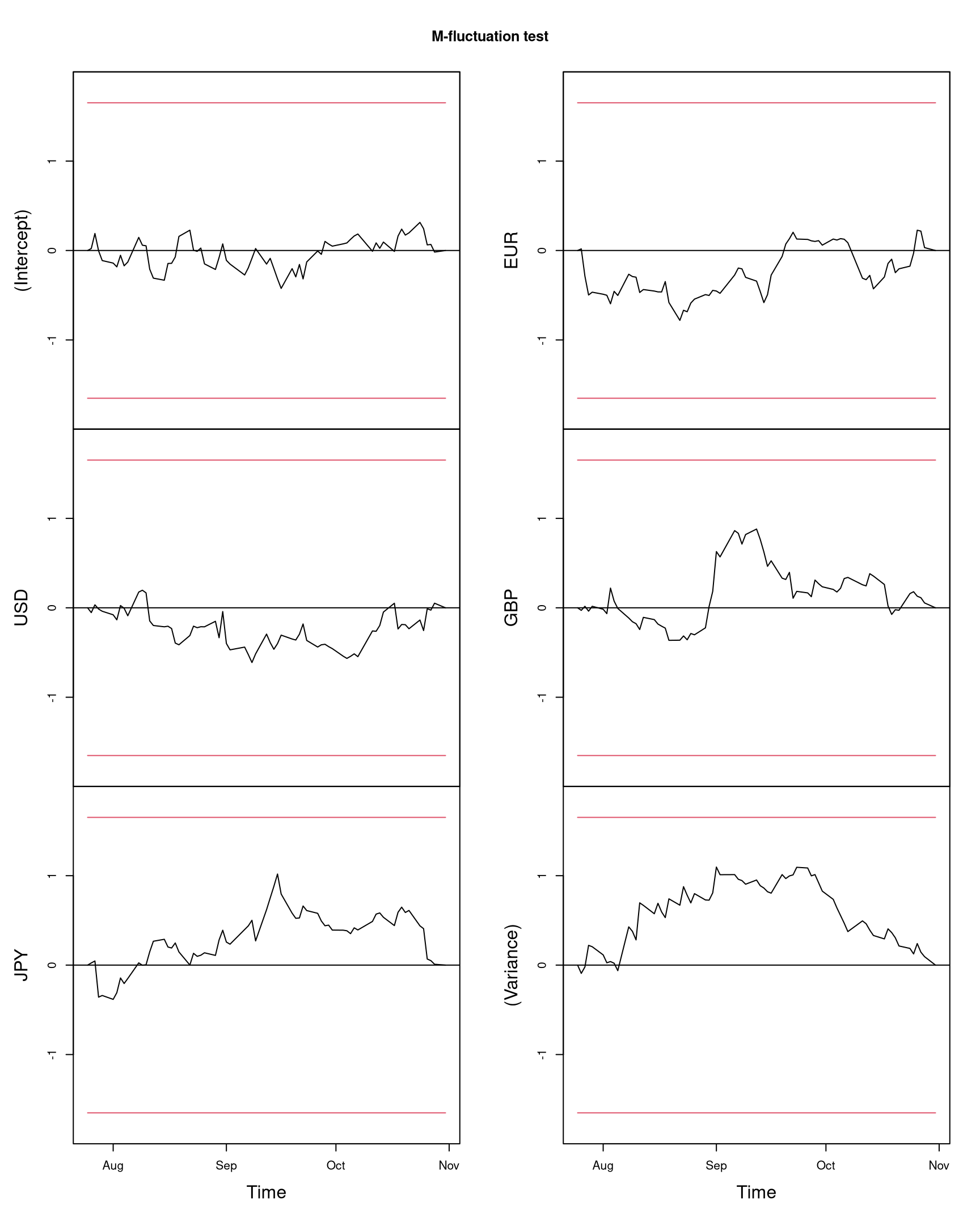
This shows that the fluctuation in the parameters during this history period is very small and non-significant:
sctest(cny_efp)
##
##  M-fluctuation test
##
## data:  cny_efp
## f(efp) = 1.0968, p-value = 0.6965
The same fluctuation process can be continued in the monitoring period to check whether future observations still conform with the established model. Using a linear boundary, derived at 5% significance level (for potentially monitoring up to \(T = 4\)), this can be performed via:
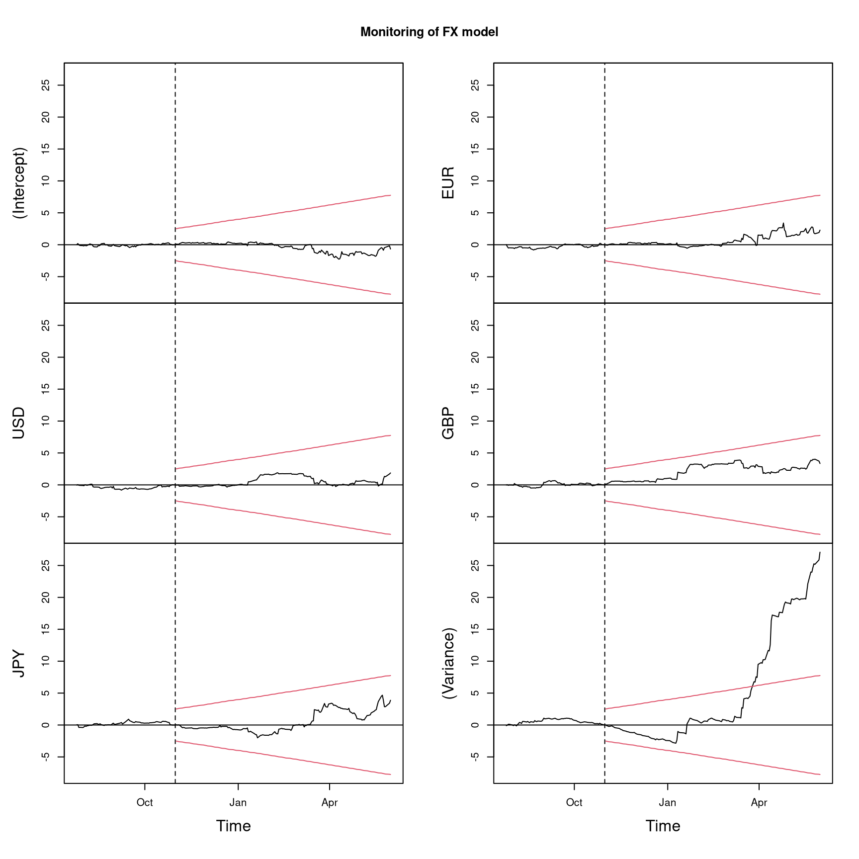
In the first months, up to spring 2006, there is still moderate fluctuation in all processes signalling no departure from the previously established USD peg. In fact, the only larger deviation during that time period is surprisingly a decrease in the variance—corresponding to a somewhat tighter USD peg—which almost leads to a boundary crossing in January 2006. However, the situation relaxes a bit before in the next weeks before in March 2006 the variance component of the fluctuation process starts to deviate clearly from its mean. However, none of the coefficients deviates from its zero mean, signalling that there was no significant change in the currency weights. The change occurs in
cny_mon
## Monitoring of FX model
##
## Formula: CNY ~ USD + JPY + EUR + GBP
## History period: 2005-07-26 to 2005-10-31
## Break detected: 2006-03-27
To capture the changes in the China’s exchange rate regime more formally, we fit a segmented exchange rate regression based on the full extended data set:
cny_reg <- fxregimes(CNY ~ USD + JPY + EUR + GBP,
  data = cny, h = 20, breaks = 10)
## [1] TRUEWe determine the optimal breakpoints for \(1, \dots, 10\) breaks with a minimal segment size of \(20\) observations and compute the associated segmented negative log-likelihood (NLL) and LWZ criterion. Both can be visualized via
plot(cny_reg)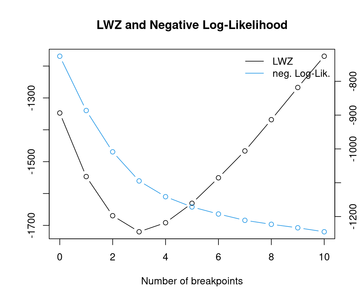
NLL decreases with every additional break but with a marked decrease only for going from 0 to 1~break. This is also reflected in the LWZ criterion that assumes its minimum for 3~break so that we choose a 3-break (or 4-segment) model. The estimated breakpoint is 2006-03-14, 2008-08-22, 2008-12-31, i.e., shortly before the boundary crossing in the monitoring procedure, confirming the findings above. The confidence interval for the break can be obtained by
confint(cny_reg, level = 0.9)
##
##   Confidence intervals for breakpoints
##   of optimal 4-segment partition:
##
## Call:
## confint.fxregimes(object = cny_reg, level = 0.9)
##
## Breakpoints at observation number:
##   5 % breakpoints 95 %
## 1 143         158  159
## 2 762         778  779
## 3 865         866  880
##
## Corresponding to breakdates:
##          5 % breakpoints       95 %
## 1 2006-02-21  2006-03-14 2006-03-15
## 2 2008-07-31  2008-08-22 2008-08-25
## 3 2008-12-30  2008-12-31 2009-01-22
showing that the end of the low variance period can be determined more precisely than the start of the high variance period. The parameter estimates for both segments can be obtained by
coef(cny_reg)
##                         (Intercept)       USD          JPY          EUR
## 2005-07-26--2006-03-14 -0.005032973 0.9994096  0.005184123 -0.015243981
## 2006-03-15--2008-08-22 -0.024992773 0.9693984 -0.009321588  0.025594292
## 2008-08-25--2008-12-31 -0.014770102 1.0307442 -0.026479209  0.048853047
## 2009-01-02--2009-07-31  0.001351404 0.9809389  0.008205345 -0.007683415
##                                 GBP   (Variance)
## 2005-07-26--2006-03-14  0.006838512 0.0007816822
## 2006-03-15--2008-08-22 -0.012867650 0.0112856274
## 2008-08-25--2008-12-31  0.007187178 0.0693969576
## 2009-01-02--2009-07-31  0.008567336 0.0019749197
A complete summary can be computed by first re-fitting the model on both sub-samples (returning a list of ``fxlm’’ objects) and then applying the usual summary():
cny_rf <- refit(cny_reg)
lapply(cny_rf, summary)
## $`2005-07-26--2006-03-14`
##
## Call:
## fxlm(formula = object$formula, data = window(object$data, start = sbp[i],
##     end = ebp[i]))
##
## Residuals:
##       Min        1Q    Median        3Q       Max
## -0.106628 -0.015830  0.001518  0.016454  0.090368
##
## Coefficients:
##              Estimate Std. Error t value Pr(>|t|)
## (Intercept) -0.005033   0.002266  -2.221   0.0278 *
## USD          0.999410   0.005421 184.370   <2e-16 ***
## JPY          0.005184   0.005230   0.991   0.3231
## EUR         -0.015244   0.016588  -0.919   0.3596
## GBP          0.006839   0.008257   0.828   0.4088
## ---
## Signif. codes:  0 '***' 0.001 '**' 0.01 '*' 0.05 '.' 0.1 ' ' 1
##
## Residual standard error: 0.02841 on 153 degrees of freedom
## Multiple R-squared:  0.9979, Adjusted R-squared:  0.9978
## F-statistic: 1.788e+04 on 4 and 153 DF,  p-value: < 2.2e-16
##
##
## $`2006-03-15--2008-08-22`
##
## Call:
## fxlm(formula = object$formula, data = window(object$data, start = sbp[i],
##     end = ebp[i]))
##
## Residuals:
##      Min       1Q   Median       3Q      Max
## -0.44652 -0.06071  0.01135  0.06138  0.45665
##
## Coefficients:
##              Estimate Std. Error t value Pr(>|t|)
## (Intercept) -0.024993   0.004300  -5.812 9.92e-09 ***
## USD          0.969398   0.011533  84.054  < 2e-16 ***
## JPY         -0.009322   0.010450  -0.892    0.373
## EUR          0.025594   0.022943   1.116    0.265
## GBP         -0.012868   0.012147  -1.059    0.290
## ---
## Signif. codes:  0 '***' 0.001 '**' 0.01 '*' 0.05 '.' 0.1 ' ' 1
##
## Residual standard error: 0.1067 on 615 degrees of freedom
## Multiple R-squared:  0.9649, Adjusted R-squared:  0.9646
## F-statistic:  4223 on 4 and 615 DF,  p-value: < 2.2e-16
##
##
## $`2008-08-25--2008-12-31`
##
## Call:
## fxlm(formula = object$formula, data = window(object$data, start = sbp[i],
##     end = ebp[i]))
##
## Residuals:
##      Min       1Q   Median       3Q      Max
## -0.97806 -0.11418 -0.01290  0.09812  0.87997
##
## Coefficients:
##              Estimate Std. Error t value Pr(>|t|)
## (Intercept) -0.014770   0.029756  -0.496    0.621
## USD          1.030744   0.043672  23.602   <2e-16 ***
## JPY         -0.026479   0.030149  -0.878    0.382
## EUR          0.048853   0.058852   0.830    0.409
## GBP          0.007187   0.035289   0.204    0.839
## ---
## Signif. codes:  0 '***' 0.001 '**' 0.01 '*' 0.05 '.' 0.1 ' ' 1
##
## Residual standard error: 0.2713 on 83 degrees of freedom
## Multiple R-squared:  0.9562, Adjusted R-squared:  0.954
## F-statistic: 452.6 on 4 and 83 DF,  p-value: < 2.2e-16
##
##
## $`2009-01-02--2009-07-31`
##
## Call:
## fxlm(formula = object$formula, data = window(object$data, start = sbp[i],
##     end = ebp[i]))
##
## Residuals:
##       Min        1Q    Median        3Q       Max
## -0.225789 -0.021239 -0.000453  0.019380  0.145003
##
## Coefficients:
##              Estimate Std. Error t value Pr(>|t|)
## (Intercept)  0.001351   0.003734   0.362   0.7179
## USD          0.980939   0.005081 193.060   <2e-16 ***
## JPY          0.008205   0.004325   1.897   0.0598 .
## EUR         -0.007683   0.009480  -0.810   0.4190
## GBP          0.008567   0.004464   1.919   0.0570 .
## ---
## Signif. codes:  0 '***' 0.001 '**' 0.01 '*' 0.05 '.' 0.1 ' ' 1
##
## Residual standard error: 0.04521 on 143 degrees of freedom
## Multiple R-squared:  0.9979, Adjusted R-squared:  0.9978
## F-statistic: 1.699e+04 on 4 and 143 DF,  p-value: < 2.2e-16
These results allow for several conclusions about the Chinese exchange rate regime after spring 2006: CNY was still closely linked to USD. The exchange rate regime got much more flexible increasing from \(\sigma = 0.028\) to \(0.106\) which is still very low, even compared with other pegged exchange rate regimes (see the results for India in vignette("INR", package = "fxregime")). The intercept was clearly smaller than 0, reflecting a slow appreciation of the CNY and thus signalling a modest liberation of the rigid USD peg in spring 2006. Towards the end of 2008, the modest liberation was abandoned again and since 2009 the exchange rate regime is again an extremely tight USD peg without appreciation.
Summary
For the Chinese yuan, a 4-segment model is found for the time after July 2005 when China gave up on a fixed exchange rate to the USD. While being closely linked to USD in all periods, there had been small steps in the direction of the claims of the Chinese central bank: flexibility slightly increased while the weight of the USD in the currency basket slightly decreased. However, these steps were reversed again towards the end of 2008.