countreg

Horseshoe Crab Mating

Description

Determinants for male satellites to nesting horseshoe crabs.

Usage

data("CrabSatellites")

Format

A data frame containing 173 observations on 5 variables.

color: Ordered factor indicating color (light medium, medium, dark medium, dark).
spine: Ordered factor indicating spine condition (both good, one worn or broken, both worn or broken).
width: Carapace width (cm).
weight: Weight (kg).
satellites: Number of satellites.

Details

Brockmann (1996) investigates horshoe crab mating. The crabs arrive on the beach in pairs to spawn. Furthermore, unattached males also come to the beach, crowd around the nesting couples and compete with attached males for fertilizations. These so-called satellite males form large groups around some couples while ignoring others. Brockmann (1996) shows that the groupings are not driven by environmental factors but by properties of the nesting female crabs. Larger females that are in better condition attract more satellites.

Agresti (2002, 2013) reanalyzes the number of satellites using count models. Explanatory variables are the female crab’s color, spine condition, weight, and carapace width. Color and spine condition are ordered factors but are treated as numeric in some analyses.

Kleiber & Zeileis (2016) employ the data for illustrating rootograms and other diagnostic graphics for various kinds of count data regression models.

Source

Table 4.3 in Agresti (2002).

References

Agresti A (2002). Categorical Data Analysis, 2nd ed., John Wiley & Sons, Hoboken.

Agresti A (2013). Categorical Data Analysis, 3rd ed., John Wiley & Sons, Hoboken.

Brockmann HJ (1996). “Satellite Male Groups in Horseshoe Crabs, Limulus polyphemus”, Ethology, 102(1), 1–21.

Kleiber C, Zeileis A (2016). “Visualizing Count Data Regressions Using Rootograms.” The American Statistician, 70(3), 296–303. doi:10.1080/00031305.2016.1173590

Examples

library("countreg")


## load data, use ordered factors as numeric, and
## grouped factor version of width
data("CrabSatellites", package = "countreg")
CrabSatellites <- transform(CrabSatellites,
  color = as.numeric(color),
  spine = as.numeric(spine),
  cwidth = cut(width, c(-Inf, seq(23.25, 29.25), Inf))
)

## Agresti, Table 4.4
aggregate(CrabSatellites$satellites, list(CrabSatellites$cwidth), function(x)
  round(c(Number = length(x), Sum = sum(x), Mean = mean(x), Var = var(x)), digits = 2))

      Group.1 x.Number  x.Sum x.Mean  x.Var
1 (-Inf,23.2]    14.00  14.00   1.00   2.77
2 (23.2,24.2]    14.00  20.00   1.43   8.88
3 (24.2,25.2]    28.00  67.00   2.39   6.54
4 (25.2,26.2]    39.00 105.00   2.69  11.38
5 (26.2,27.2]    22.00  63.00   2.86   6.89
6 (27.2,28.2]    24.00  93.00   3.88   8.81
7 (28.2,29.2]    18.00  71.00   3.94  16.88
8 (29.2, Inf]    14.00  72.00   5.14   8.29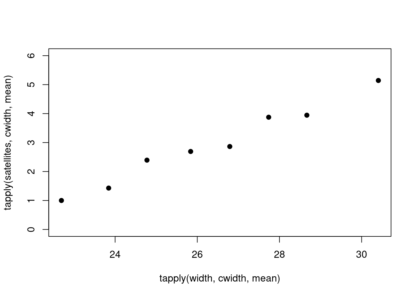

## Agresti, Figure 4.4
plot(tapply(satellites, cwidth, mean) ~ tapply(width, cwidth, mean),
  data = CrabSatellites, ylim = c(0, 6), pch = 19)

## alternatively: exploratory displays for hurdle (= 0 vs. > 0) and counts (> 0)
par(mfrow = c(2, 2))
plot(factor(satellites == 0) ~ width, data = CrabSatellites, breaks = seq(20, 33.5, by = 1.5))
plot(factor(satellites == 0) ~ color, data = CrabSatellites, breaks = 1:5 - 0.5)
plot(jitter(satellites) ~ width, data = CrabSatellites, subset = satellites > 0, log = "y")
plot(jitter(satellites) ~ factor(color), data = CrabSatellites, subset = satellites > 0, log = "y")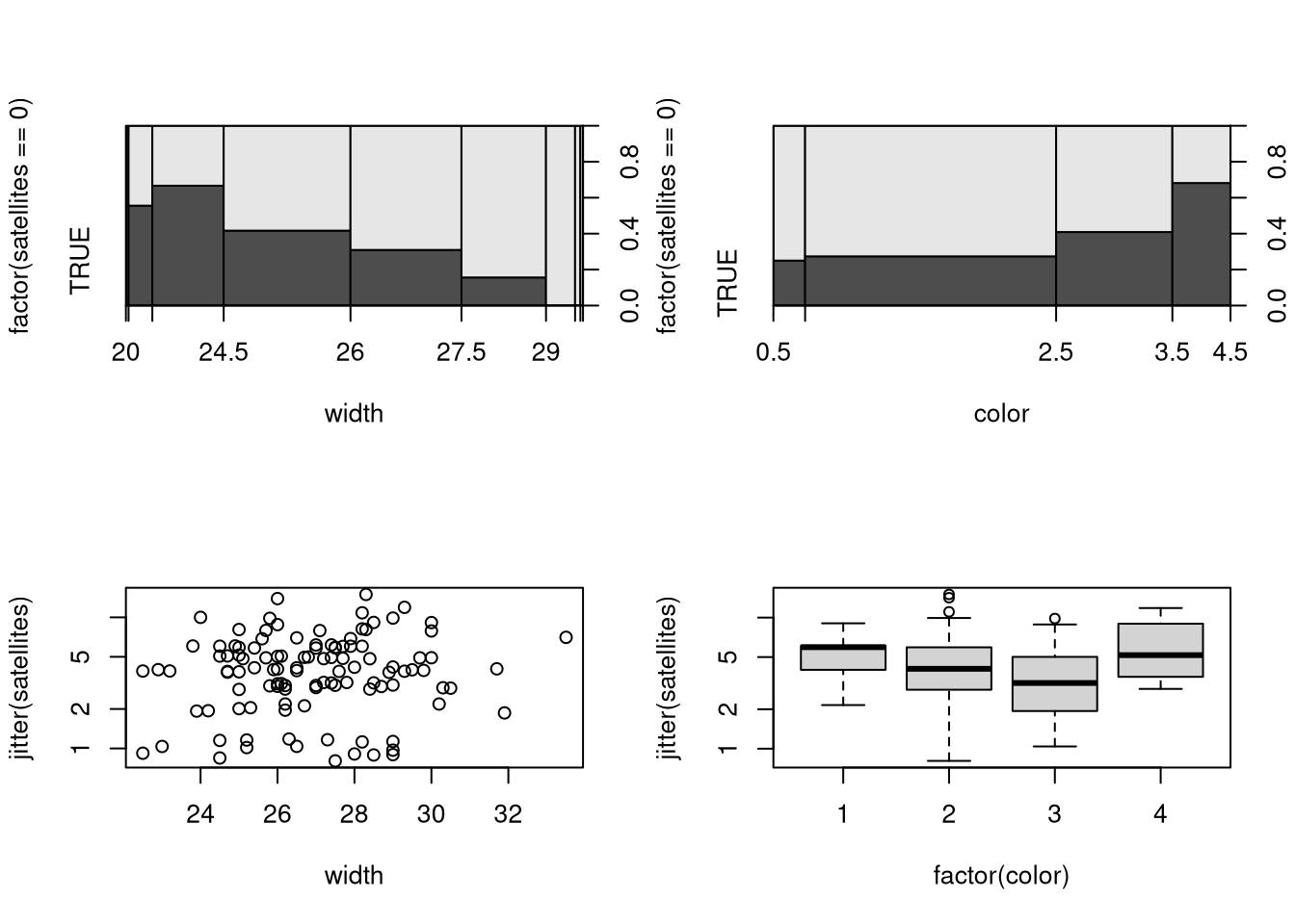

## count data models
cs_p    <-    glm(satellites ~ width + color, data = CrabSatellites, family = poisson)
cs_nb   <- glm.nb(satellites ~ width + color, data = CrabSatellites)
cs_hp   <- hurdle(satellites ~ width + color, data = CrabSatellites, dist = "poisson")
cs_hnb  <- hurdle(satellites ~ width + color, data = CrabSatellites, dist = "negbin")
cs_hnb2 <- hurdle(satellites ~ 1 | width + color, data = CrabSatellites, dist = "negbin")
AIC(cs_p, cs_nb, cs_hp, cs_hnb, cs_hnb2)

        df      AIC
cs_p     3 921.4990
cs_nb    4 756.9323
cs_hp    6 736.2160
cs_hnb   7 714.7255
cs_hnb2  5 712.0658

BIC(cs_p, cs_nb, cs_hp, cs_hnb, cs_hnb2)

        df      BIC
cs_p     3 930.9589
cs_nb    4 769.5455
cs_hp    6 755.1358
cs_hnb   7 736.7985
cs_hnb2  5 727.8323

## rootograms (Kleiber & Zeileis, Figure 2)
library("topmodels")
par(mfrow = c(2, 2))
r_p   <- rootogram(cs_p,   xlim = c(0, 15), main = "Poisson")
r_nb  <- rootogram(cs_nb,  xlim = c(0, 15), main = "Negative Binomial")
r_hp  <- rootogram(cs_hp,  xlim = c(0, 15), main = "Hurdle Poisson")
r_hnb <- rootogram(cs_hnb, xlim = c(0, 15), main = "Hurdle Negative Binomial")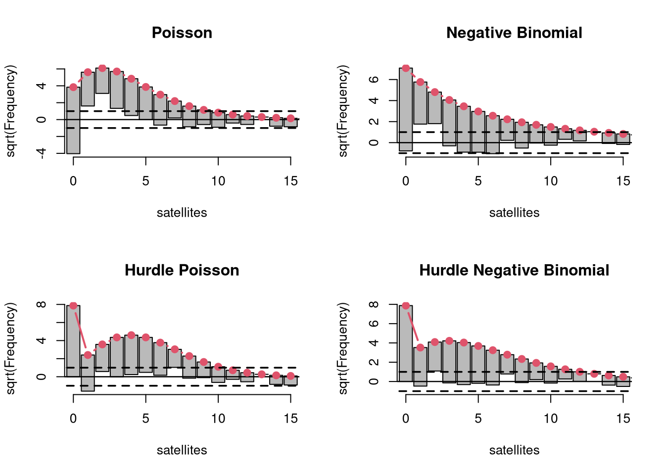

## fitted curves (Kleiber & Zeileis, Figure 4)
par(mfrow = c(1, 1))
plot(jitter(satellites) ~ width, data = CrabSatellites)
nd <- data.frame(width = 20:34, color = 2)
pred <- function(m) predict(m, newdata = nd, type = "response")
cs_ag <- glm(satellites ~ width, data = CrabSatellites, family = poisson(link = "identity"),
  start = coef(lm(satellites ~ width, data = CrabSatellites)))
lines(pred(cs_ag)   ~ width, data = nd, col = 2, lwd = 1.5)
lines(pred(cs_p)    ~ width, data = nd, col = 3, lwd = 1.5)
lines(pred(cs_hnb)  ~ width, data = nd, col = 4, lwd = 1.5)
lines(pred(cs_hnb2) ~ width, data = nd, col = 4, lwd = 1.5, lty = 2)
legend("topleft", c("Hurdle NB", "Hurdle NB 2", "Poisson (id)", "Poisson (log)"),
  col = c(4, 4, 2, 3), lty = c(1, 2, 1, 1), lwd = 1.5, bty = "n")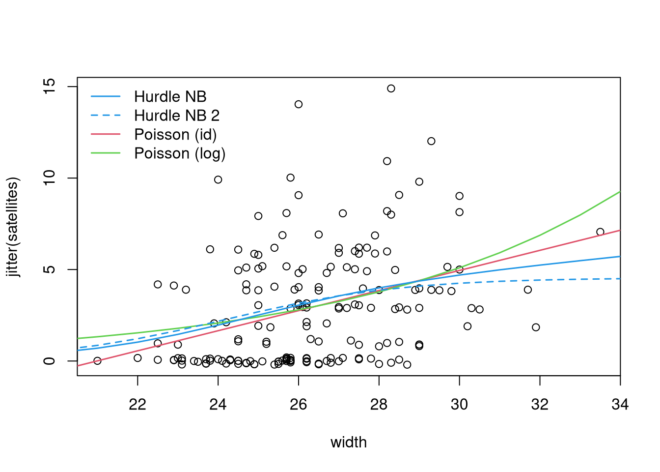

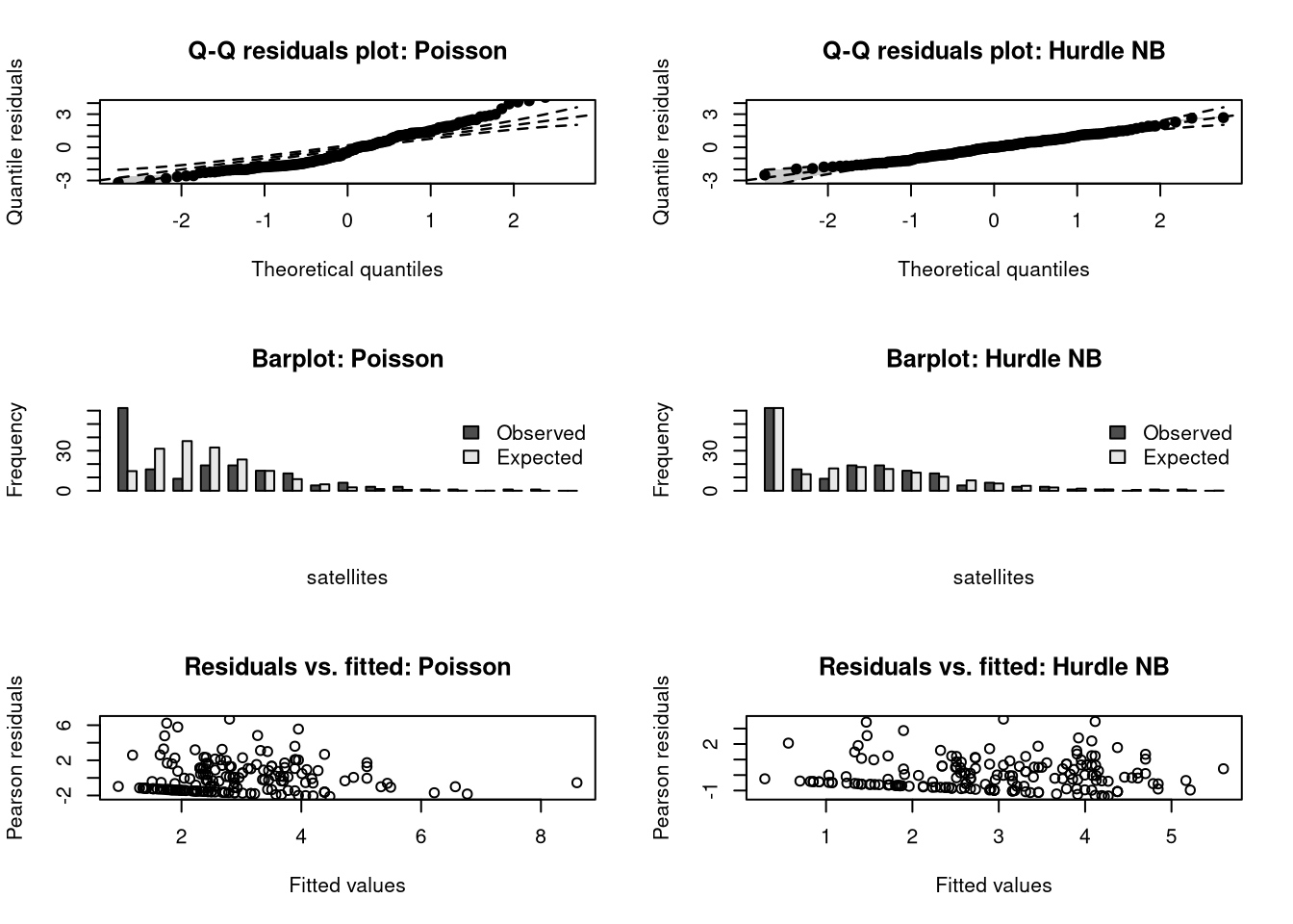
## alternative displays (Kleiber & Zeileis, Figure 3):
## Q-Q residuals plot, barplot, residuals vs. fitted
par(mfrow= c(3, 2))
qqrplot(cs_p,   main = "Q-Q residuals plot: Poisson",   ylim = c(-3, 4))
qqrplot(cs_hnb, main = "Q-Q residuals plot: Hurdle NB", ylim = c(-3, 4))

barplot(t(matrix(c(r_p$observed, r_p$expected)^2, ncol = 2,
  dimnames = list(r_p$x, c("Observed", "Expected")))),
  beside = TRUE, main = "Barplot: Poisson",
  xlab = "satellites", ylab = "Frequency",
  legend.text = TRUE, args.legend = list(x = "topright", bty = "n"))
barplot(t(matrix(c(r_hnb$observed, r_hnb$expected)^2, ncol = 2,
  dimnames = list(r_hnb$x, c("Observed", "Expected")))),
  beside = TRUE, main = "Barplot: Hurdle NB",
  xlab = "satellites", ylab = "Frequency",
  legend.text = TRUE, args.legend = list(x = "topright", bty = "n"))

plot(predict(cs_p, type = "response"),
  residuals(cs_p, type = "pearson"),
  xlab = "Fitted values", ylab = "Pearson residuals",
  main = "Residuals vs. fitted: Poisson")
plot(predict(cs_hnb, type = "response"),
  residuals(cs_hnb, type = "pearson"),
  xlab = "Fitted values", ylab = "Pearson residuals",
  main = "Residuals vs. fitted: Hurdle NB")