(No) Myopic Loss Aversion in Adolescents

Description

Data from a behavioral economics experiment assessing the extent of myopic loss aversion among adolescents (mostly aged 11 to 19).

Usage

data("LossAversion", package = "betareg")

Format

A data frame containing 570 observations on 7 variables.

invest

numeric. Average proportion of tokens invested across all 9 rounds.

gender

factor. Gender of the player (or team of players).

male

factor. Was (at least one of) the player(s) male (in the team)?

age

numeric. Age in years (averaged for teams).

treatment

factor. Type of treatment: long vs. short.

grade

factor. School grades: 6-8 (11-14 years) vs. 10-12 (15-18 years).

arrangement

factor. Is the player a single player or team of two?

Details

Myopic loss aversion is a phenomenon in behavioral economics, where individuals do not behave economically rationally when making short-term decisions under uncertainty. Example: In lotteries with positive expected payouts investments are lower than the maximum possible (loss aversion). This effect is enhanced for short-term investments (myopia or short-sightedness).

The data in LossAversion were collected by Matthias Sutter and Daniela Glätzle-Rützler (Universität Innsbruck) in an experiment with high-school students in Tyrol, Austria (Schwaz and Innsbruck). The students could invest X tokens (0-100) in each of 9 rounds in a lottery. The payouts were 100 + 2.5 * X tokens with probability 1/3 and 100 - X tokens with probability 2/3. Thus, the expected payouts were 100 + 1/6 * X tokens. Depending on the treatment in the experiment, the investments could either be modified in each round (treatment: "short") or only in round 1, 4, 7 (treatment "long"). Decisions were either made alone or in teams of two. The tokens were converted to monetary payouts using a conversion of EUR 0.5 per 100 tokens for lower grades (Unterstufe, 6-8) or EUR 1.0 per 100 tokens for upper grades (Oberstufe, 10-12).

From the myopic loss aversion literature (on adults) one would expect that the investments of the players (either single players or teams of two) would depend on all factors: Investments should be

• lower in the short treatment (which would indicate myopia),

• higher for teams (indicating a reduction in loss aversion),

• higher for (teams with) male players,

• increase with age/grade.

See Glätzle-Rützler et al. (2015) for more details and references to the literature. In their original analysis, the investments are analyzes using a panel structure (i.e., 9 separate investments for each team). Here, the data are averaged across rounds for each player, leading to qualitatively similar results. The full data along with replication materials are available in the Harvard Dataverse.

Kosmidis and Zeileis (2026) revisit the data using extended-support beta mixture (XBX) regression, which can simultaneously capture both the probability of rational behavior and the mean amount of loss aversion.

Source

Glätzle-Rützler D, Sutter M, Zeileis A (2020). Replication Data for: No Myopic Loss Aversion in Adolescents? - An Experimental Note. Harvard Dataverse, UNF:6:6hVtbHavJAFYfL7dDl7jqA==. doi:10.7910/DVN/IHFZAK

References

Glätzle-Rützler D, Sutter M, Zeileis A (2015). No Myopic Loss Aversion in Adolescents? – An Experimental Note. Journal of Economic Behavior & Organization, 111, 169–176. doi:10.1016/j.jebo.2014.12.021

Kosmidis I, Zeileis A (2026). Extended-Support Beta Regression for [0, 1] Responses. Journal of the Royal Statistical Society C, 75(1), 139–157. doi:10.1093/jrsssc/qlaf039

See Also

betareg

Examples

library("betareg")

options(digits = 4)

## data and add ad-hoc scaling (a la Smithson & Verkuilen)
data("LossAversion", package = "betareg")
LossAversion <- transform(LossAversion,
  invests = (invest * (nrow(LossAversion) - 1) + 0.5)/nrow(LossAversion))


## models: normal (with constant variance), beta, extended-support beta mixture
la_n <- lm(invest ~ grade * (arrangement + age) + male, data = LossAversion)
summary(la_n)

Call:
lm(formula = invest ~ grade * (arrangement + age) + male, data = LossAversion)

Residuals:
    Min      1Q  Median      3Q     Max 
-0.7735 -0.1967  0.0024  0.1916  0.5724 

Coefficients:
                           Estimate Std. Error t value Pr(>|t|)    
(Intercept)                  0.2844     0.1575    1.81  0.07136 .  
grade10-12                  -0.8437     0.2815   -3.00  0.00284 ** 
arrangementteam              0.0628     0.0302    2.08  0.03788 *  
age                          0.0115     0.0124    0.93  0.35041    
maleyes                      0.1035     0.0232    4.46  9.9e-06 ***
grade10-12:arrangementteam   0.1507     0.0455    3.32  0.00097 ***
grade10-12:age               0.0458     0.0185    2.47  0.01380 *  
---
Signif. codes:  0 '***' 0.001 '**' 0.01 '*' 0.05 '.' 0.1 ' ' 1

Residual standard error: 0.247 on 563 degrees of freedom
Multiple R-squared:  0.158, Adjusted R-squared:  0.149 
F-statistic: 17.7 on 6 and 563 DF,  p-value: <2e-16

la_b <- betareg(invests ~ grade * (arrangement + age) + male | arrangement + male + grade,
  data = LossAversion)
summary(la_b)

Call:
betareg(formula = invests ~ grade * (arrangement + age) + male | arrangement + 
    male + grade, data = LossAversion)

Quantile residuals:
   Min     1Q Median     3Q    Max 
-3.948 -0.594 -0.042  0.554  4.439 

Coefficients (mean model with logit link):
                           Estimate Std. Error z value Pr(>|z|)    
(Intercept)                 -1.4139     0.6197   -2.28   0.0225 *  
grade10-12                  -2.9435     1.2520   -2.35   0.0187 *  
arrangementteam              0.2250     0.1175    1.92   0.0554 .  
age                          0.0906     0.0486    1.87   0.0621 .  
maleyes                      0.4553     0.0990    4.60  4.2e-06 ***
grade10-12:arrangementteam   0.6549     0.2003    3.27   0.0011 ** 
grade10-12:age               0.1513     0.0806    1.88   0.0605 .  

Phi coefficients (precision model with log link):
                Estimate Std. Error z value Pr(>|z|)    
(Intercept)        1.194      0.084   14.21  < 2e-16 ***
arrangementteam    0.406      0.122    3.33  0.00087 ***
maleyes           -0.555      0.113   -4.93  8.2e-07 ***
grade10-12        -0.553      0.104   -5.31  1.1e-07 ***
---
Signif. codes:  0 '***' 0.001 '**' 0.01 '*' 0.05 '.' 0.1 ' ' 1 

Type of estimator: ML (maximum likelihood)
Log-likelihood: 94.4 on 11 Df
Pseudo R-squared: 0.154
Number of iterations: 24 (BFGS) + 3 (Fisher scoring) 

la_xbx <- betareg(invest ~ grade * (arrangement + age) + male | arrangement + male + grade,
  data = LossAversion)
summary(la_xbx)

Call:
betareg(formula = invest ~ grade * (arrangement + age) + male | arrangement + 
    male + grade, data = LossAversion)

Randomized quantile residuals:
   Min     1Q Median     3Q    Max 
-3.084 -0.693 -0.015  0.698  3.083 

Coefficients (mu model with logit link):
                           Estimate Std. Error z value Pr(>|z|)    
(Intercept)                 -0.8650     0.5193   -1.67  0.09577 .  
grade10-12                  -3.0962     1.0529   -2.94  0.00328 ** 
arrangementteam              0.2079     0.0987    2.11  0.03508 *  
age                          0.0489     0.0406    1.20  0.22857    
maleyes                      0.3792     0.0842    4.50  6.6e-06 ***
grade10-12:arrangementteam   0.5672     0.1690    3.36  0.00079 ***
grade10-12:age               0.1687     0.0677    2.49  0.01275 *  

Phi coefficients (phi model with log link):
                Estimate Std. Error z value Pr(>|z|)    
(Intercept)        1.756      0.128   13.70  < 2e-16 ***
arrangementteam    0.325      0.145    2.25  0.02446 *  
maleyes           -0.484      0.136   -3.56  0.00037 ***
grade10-12        -0.316      0.131   -2.41  0.01608 *  

Exceedence parameter (extended-support xbetax model):
        Estimate Std. Error z value Pr(>|z|)    
Log(nu)   -2.273      0.245   -9.27   <2e-16 ***
---
Signif. codes:  0 '***' 0.001 '**' 0.01 '*' 0.05 '.' 0.1 ' ' 1 

Exceedence parameter nu: 0.103
Type of estimator: ML (maximum likelihood)
Log-likelihood: -71.8 on 12 Df
Number of iterations in BFGS optimization: 45 

## coefficients in XBX are typically somewhat shrunken compared to beta
cbind(XBX = coef(la_xbx), Beta = c(coef(la_b), NA))

                                XBX     Beta
(Intercept)                -0.86495 -1.41389
grade10-12                 -3.09624 -2.94347
arrangementteam             0.20790  0.22498
age                         0.04889  0.09061
maleyes                     0.37925  0.45534
grade10-12:arrangementteam  0.56724  0.65487
grade10-12:age              0.16866  0.15129
(phi)_(Intercept)           1.75629  1.19429
(phi)_arrangementteam       0.32525  0.40631
(phi)_maleyes              -0.48406 -0.55481
(phi)_grade10-12           -0.31593 -0.55271
Log(nu)                    -2.27289       NA

## predictions on subset: (at least one) male players, higher grades, around age 16
la <- subset(LossAversion, male == "yes" & grade == "10-12" & age >= 15 &  age <= 17)
la_nd <- data.frame(arrangement = c("single", "team"), male = "yes", age = 16, grade = "10-12")

## empirical vs fitted E(Y)
la_nd$mean_emp <- aggregate(invest ~ arrangement, data = la, FUN = mean)$invest 
la_nd$mean_n <- predict(la_n, la_nd)
la_nd$mean_b <- predict(la_b, la_nd)
la_nd$mean_xbx <- predict(la_xbx, la_nd)
la_nd

  arrangement male age grade mean_emp mean_n mean_b mean_xbx
1      single  yes  16 10-12   0.4824 0.4612 0.4921   0.4713
2        team  yes  16 10-12   0.6648 0.6747 0.7002   0.6861

## visualization: all means rather similar
la_mod <- c("Emp", "N", "B", "XBX")
la_col <- unname(palette.colors())[c(1, 2, 4, 4)]
la_lty <- c(1, 5, 5, 1)
matplot(la_nd[, paste0("mean_", tolower(la_mod))], type = "l",
  col = la_col, lty = la_lty, lwd = 2, ylab = "E(Y)", main = "E(Y)", xaxt = "n")
axis(1, at = 1:2, labels = la_nd$arrangement)
legend("topleft", la_mod, col = la_col, lty = la_lty, lwd = 2, bty = "n")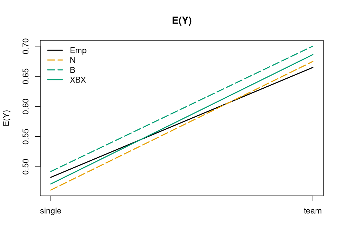

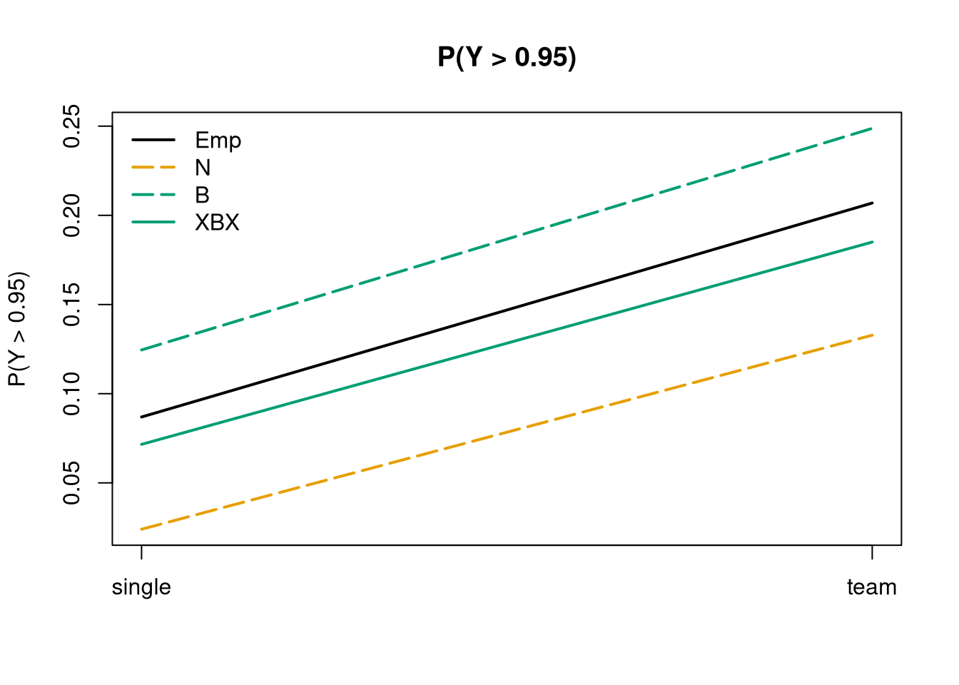
## empirical vs. fitted P(Y > 0.95)
la_nd$prob_emp <- aggregate(invest >= 0.95 ~ arrangement, data = la, FUN = mean)$invest
la_nd$prob_n <- pnorm(0.95, mean = la_nd$mean_n, sd = summary(la_n)$sigma, lower.tail = FALSE)
la_nd$prob_b <- 1 - predict(la_b, la_nd, type = "probability", at = 0.95)
la_nd$prob_xbx <- 1 - predict(la_xbx, la_nd, type = "probability", at = 0.95)
la_nd[, -(5:8)]

  arrangement male age grade prob_emp  prob_n prob_b prob_xbx
1      single  yes  16 10-12  0.08696 0.02403 0.1245  0.07161
2        team  yes  16 10-12  0.20690 0.13280 0.2487  0.18501

## visualization: only XBX works well
matplot(la_nd[, paste0("prob_", tolower(la_mod))], type = "l",
  col = la_col, lty = la_lty, lwd = 2, ylab = "P(Y > 0.95)", main = "P(Y > 0.95)", xaxt = "n")
axis(1, at = 1:2, labels = la_nd$arrangement)
legend("topleft", la_mod, col = la_col, lty = la_lty, lwd = 2, bty = "n")