Chi-Squared Automatic Interaction Detection (CHAID)

Overview

The R package chaid is an implementation of CHAID, a type of decision tree technique for a nominal dependent variable published in 1980 by Gordon V. Kass. CHAID stands for Chi-Squared Automatic Interaction Detection and detects interactions between categorized variables of a data set, one of which is the dependent variable. The remaining variables may or may not be ordered. An algorithm for recursive partitioning is implemented, based on maximizing the significance of a chi-squared statistic for cross-tabulations between the dependent variable and the predictors at each partition. The data are partitioned into mutually exclusive, exhaustive subsets that best describe the dependent variable. Multiway splits are used by default.

Installation

The chaid package is available from R-universe:

install.packages("chaid", repos = "https://zeileis.R-universe.dev")

License

The package is available under the General Public License version 2

Get started

To illustrate the chaid package, we model survival on board of the RMS Titanic by gender (male vs. female), age (adult vs. child), and travel class (1st, 2nd, 3rd, crew). The data is available in tabular form in base R and is reshaped here to a data frame with four columns and 2201 rows.

library("chaid")
data("Titanic", package = "datasets")
ttnc <- as.data.frame(Titanic)
ttnc <- ttnc[rep(1:nrow(ttnc), ttnc$Freq), 1:4]

The CHAID tree can then be fitted, printed, and visualized by:

tr <- chaid(Survived ~ ., data = ttnc)
print(tr)
## 
## Model formula:
## Survived ~ Class + Sex + Age
## 
## Fitted party:
## [1] root
## |   [2] Sex in Male
## |   |   [3] Age in Child
## |   |   |   [4] Class in 1st, 2nd, Crew: Yes (n = 16, err = 0.0%)
## |   |   |   [5] Class in 3rd: No (n = 48, err = 27.1%)
## |   |   [6] Age in Adult
## |   |   |   [7] Class in 1st: No (n = 175, err = 32.6%)
## |   |   |   [8] Class in 2nd: No (n = 168, err = 8.3%)
## |   |   |   [9] Class in 3rd: No (n = 462, err = 16.2%)
## |   |   |   [10] Class in Crew: No (n = 862, err = 22.3%)
## |   [11] Sex in Female
## |   |   [12] Class in 1st: Yes (n = 145, err = 2.8%)
## |   |   [13] Class in 2nd, Crew: Yes (n = 129, err = 12.4%)
## |   |   [14] Class in 3rd: No (n = 196, err = 45.9%)
## 
## Number of inner nodes:    5
## Number of terminal nodes: 9
plot(tr)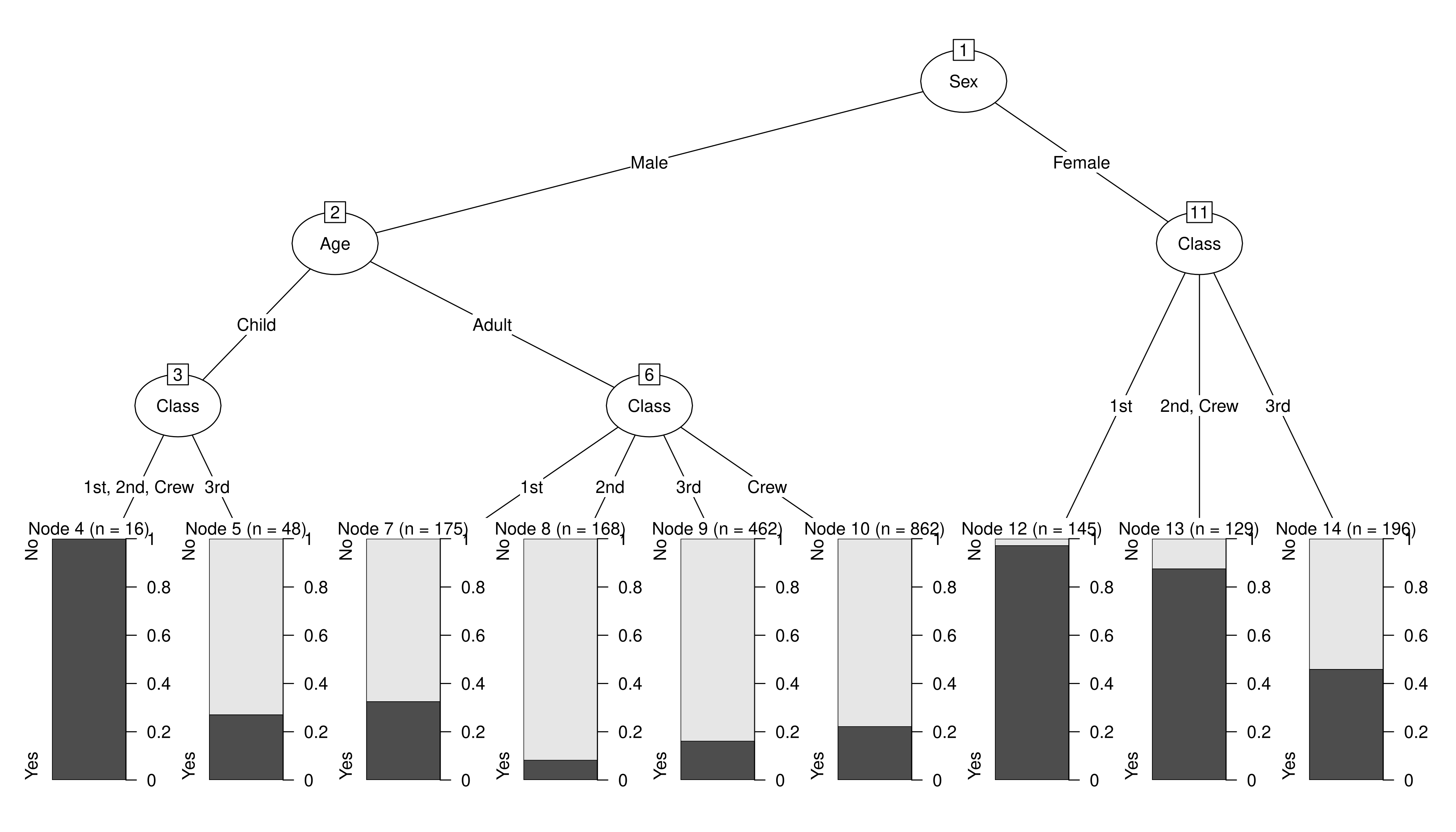

To illustrate how different types of predictions can be obtained, we set up a small example data frame for all possible combinations of gender and age in the 1st class. Clearly, “women and children first” has been applied in this class.

class1 <- expand.grid(
  Class = "1st",
  Sex = c("Male", "Female"),
  Age = c("Adult", "Child")
)
class1$response <- predict(tr, newdata = class1, type = "response")
class1$prob <- predict(tr, newdata = class1, type = "prob")
class1
##   Class    Sex   Age response    prob.No   prob.Yes
## 1   1st   Male Adult       No 0.67428571 0.32571429
## 2   1st Female Adult      Yes 0.02758621 0.97241379
## 3   1st   Male Child      Yes 0.00000000 1.00000000
## 4   1st Female Child      Yes 0.02758621 0.97241379